

In Module 12
Aufgaben
Introduction to switching operations

The transfer element (two-stage) shown on the right is given. The transient behaviour of the voltage \(u_2\) at the
output is examined when an ideal DC voltage source is connected. \(U_q\).
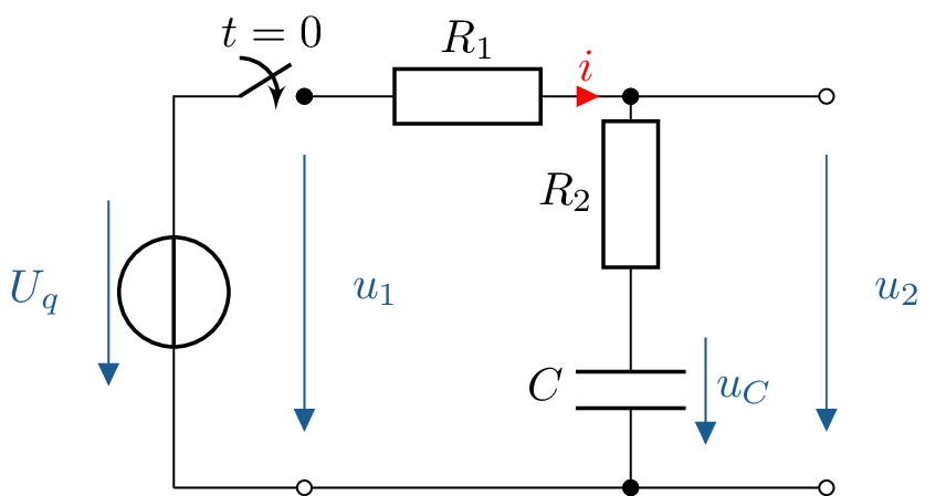
The switch-on behaviour of the circuit shown is to be investigated.
At time \(t = 0\), the switch is flipped so that the DC voltage \(U_q\) is applied to the circuit. The capacitance is completely discharged before the switching point.
a) Initial state (\(t \geq 0\)): \(U_q\) applied to the circuit: \(R_1\) in series with a parallel combination of \(R_2\) and \(C\).
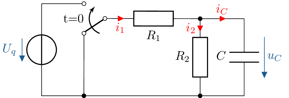
1. Set up the differential equation for \(u_C\) (\(t \geq 0\)) \begin {align*} u_{R1} + u_C &= U_q & u_{R_1} &= R_1 \cdot i_{R1}\\ R_1 \cdot i_{R1} + u_C &= U_q & i_{R1} &= i_{R2} + i_C\\ R_1 \cdot (i_C + i_{R2}) + u_C &= U_q & i_C &= C \cdot \mathrm{d}t \, u_C \qquad i_{R2} = \frac {u_C}{R_2}\\ C \cdot R_1 \cdot \mathrm{d}t \, u_C + \frac {R_1}{R_2} \cdot u_C + u_C &= U_q &&\Big | \cdot R_2\\ C \cdot R_1 \cdot R_2 \cdot \mathrm{d}t \, u_C + \left (R_1 + R_2 \right ) \cdot u_C &= U_q \cdot R_2 &&\Big | : (R_1+R_2)\\ \underbrace {C \cdot \frac {R_1 \cdot R_2}{R_1+R_2}}_{\tau } \cdot \mathrm{d}t \, u_C + u_C &= U_q \cdot \frac {R_2}{R_1+R_2} \end {align*}
2. Homogeneous solution and 3. Particulate solution (\(t \to \infty \)) \begin {align*} u_{C,h} &= K \cdot \mathrm {e}^{\lambda t} = K \cdot \mathrm {e}^{-\frac {t}{\tau }} & \tau &= C \cdot \frac {R_1 \cdot R_2}{R_1+R_2} \\[2pt] u_{C,p} &= U_q \cdot \frac {R_2}{R_1+R_2} & &\text {$C$ entspricht Leerlauf} \end {align*}
4. Determine superposition and 5th constant \(K\) \begin {align*} u_C(t) = u_{C,h} + u_{C,p} &= K \cdot \mathrm {e}^{-\frac {t}{\tau }} + U_q \cdot \frac {R_2}{R_1+R_2} \\ u_C(0) &= K \cdot \cancel {\mathrm {e}^{0}} + U_q \cdot \frac {R_2}{R_1+R_2} \overset {!}{=} 0 & \Rightarrow K &= -U_q \cdot \frac {R_2}{R_1+R_2} \\ u_C(t) &= U_q \cdot \frac {R_2}{R_1+R_2} \cdot \left ( 1 - \mathrm {e}^{-\frac {t}{\tau }} \right ) \end {align*}
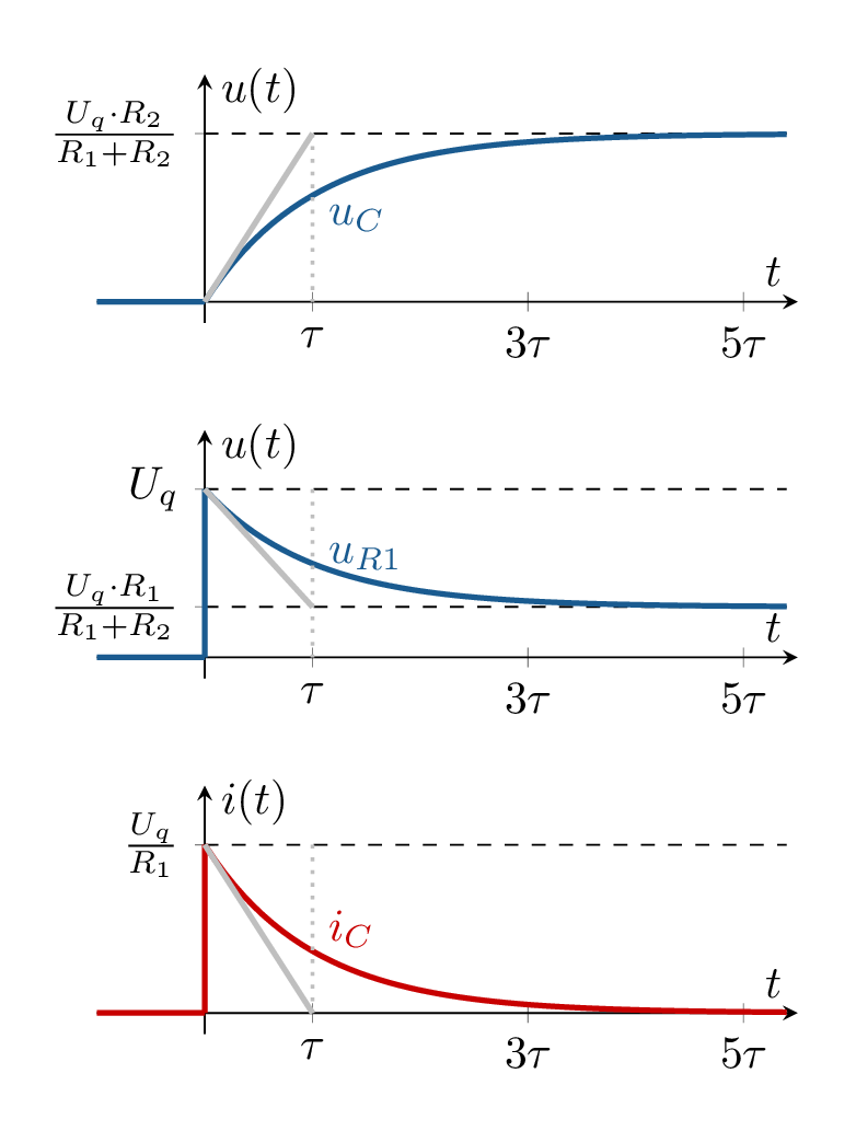
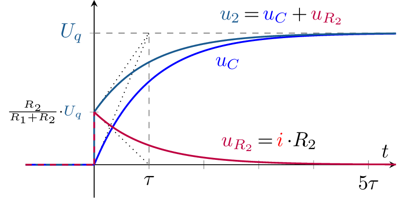
b) Sketch \(u_C(t)\), \(u_{R_1}\) and \(i_C\) with \(u_C(t)\) from a): \begin {align*} u_{R1}(t) &= U_q - u_C(t) \\ &= U_q - U_q \cdot \frac {R_2}{R_1+R_2} \cdot \left ( 1 - \mathrm {e}^{-\frac {t}{\tau }} \right ) \\ &= U_q \cdot \frac {R_1}{R_1+R_2} + U_q \cdot \frac {R_2}{R_1+R_2} \cdot \mathrm {e}^{-\frac {t}{\tau }} \\[4pt] i_C(t) &= C \cdot \mathrm{d}t \, u_C(t) \\ &= C \cdot U_q \cdot \frac {R_2}{R_1+R_2} \cdot \frac {1}{\tau } \cdot \mathrm {e}^{-\frac {t}{\tau }} \\ &= U_q \cdot \frac {\cancel {C} \cdot \cancel {R_2}}{\cancel {R_1+R_2}} \cdot \frac {\cancel {R_1+R_2}}{\cancel {C} \cdot R_1 \cdot \cancel {R_2}} \cdot \mathrm {e}^{-\frac {t}{\tau }}\\ &= \frac {U_q}{R_1} \cdot \mathrm {e}^{-\frac {t}{\tau }} \end {align*}
The switching behaviour of the circuit shown in the left-hand figure is to be investigated.
The voltage curve \(u_1(t)\) is shown in the right-hand figure.
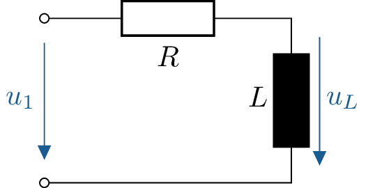
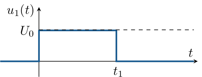
Before time \(t=0\), the voltage \(u_1 = 0\), so that at time \(t=0\) no energy is stored in the coil. Furthermore, \(t_1 \gg 5\tau \).
Continue to consider the charging process. Now: \(R = 5\,\Omega \), \(L=100\,\text {mH}\), and \(U_0=2.8\,\text {kV}\).
\begin {align*} \text {ODE (general):}&& \frac {L}{R}\cdot \mathrm{d}t \, i &= \frac {U_1}{R_1} \text {(Switch on)}\\ \text {Solution approach:}&& i &= \frac {U_0}{R}\cdot (1-e^{-\frac {t}{\tau }}) \text {with} \tau =\frac {L}{R} \end {align*}
a) Calculate inductance.
\(\tau =\frac {L}{R}\) \(L=\tau \cdot R=1\,ms\cdot 100\,\Omega =0,1\,H\)
b) Charging process, coil current \(i_L\) at time \(t=3\tau \).\begin {align*} i(t=3\cdot \tau ) &= \frac {U_0}{R}(1-e^{-\frac {t}{\tau }})\\ &=\frac {1\,kV}{100\,\Omega }\cdot (1-e^{-3}) = 10\,A\cdot 0,95\\ &=9,5\,A \end {align*}
c) Time until completion of the settling process, coil current and voltage after \(50\,ms\).\begin {align*} \tau &=\frac {L}{R}=\frac {0,1\,H}{5\,\Omega }=0,02\,s=20\,ms\\\\ i(t=50\,ms)&=\frac {U_0}{R}\cdot (1-e^{-\frac {t}{\tau }})\\ &=\frac {2,8\,kV}{5\,\Omega }\cdot (1-e^{-\frac {50\,ms}{20\,ms}})\\ &=0,56\,kA\cdot (0,918)=0,514\,kA\\\\ u_L&=L\cdot \mathrm{d}t i_L = \frac {L}{R}\cdot U_0 \cdot (-\frac {1}{\tau })\cdot (-e^{-\frac {t}{\tau }})\\ &= U_0\cdot e^{-\frac {t}{\tau }}\\\\ u_L(t=50\,ms)&=2,8\,kV\cdot e^{-\frac {50\,ms}{20\,ms}}=229,8\,V\\ t_0&=5\cdot \tau =5\cdot 20\,ms=100\,ms \end {align*}
d) Discharge process, coil current and voltage after \(t = t_1 + 50\,ms\).\begin {align*} \text {ODE (Unloading process):}&& \frac {L}{R}\cdot \mathrm{d}t \, i+i &=0\\ \text {Approach to a solution:}&& i &= \frac {U_0}{R}\cdot e^{-\frac {t}{\tau }} \text {mit} \tau =\frac {L}{R}\\ \end {align*}
\begin {align*} u_L&=L\cdot \mathrm{d}t i = \frac {L}{R}\cdot u_0\cdot (-\frac {1}{\tau })\cdot e^{-\frac {t}{\tau }}\\ &=-U_0\cdot e^{-\frac {t}{\tau }}\\ i(50\,ms)&=\frac {2,8\,kV}{5\Omega }\cdot e^{-\frac {50\,ms}{20\,ms}}=46\,A\\ u_L(50\,ms)&=-2,8\,kV\cdot e^{-\frac {50\,ms}{20\,ms}}=-230\,V \end {align*}
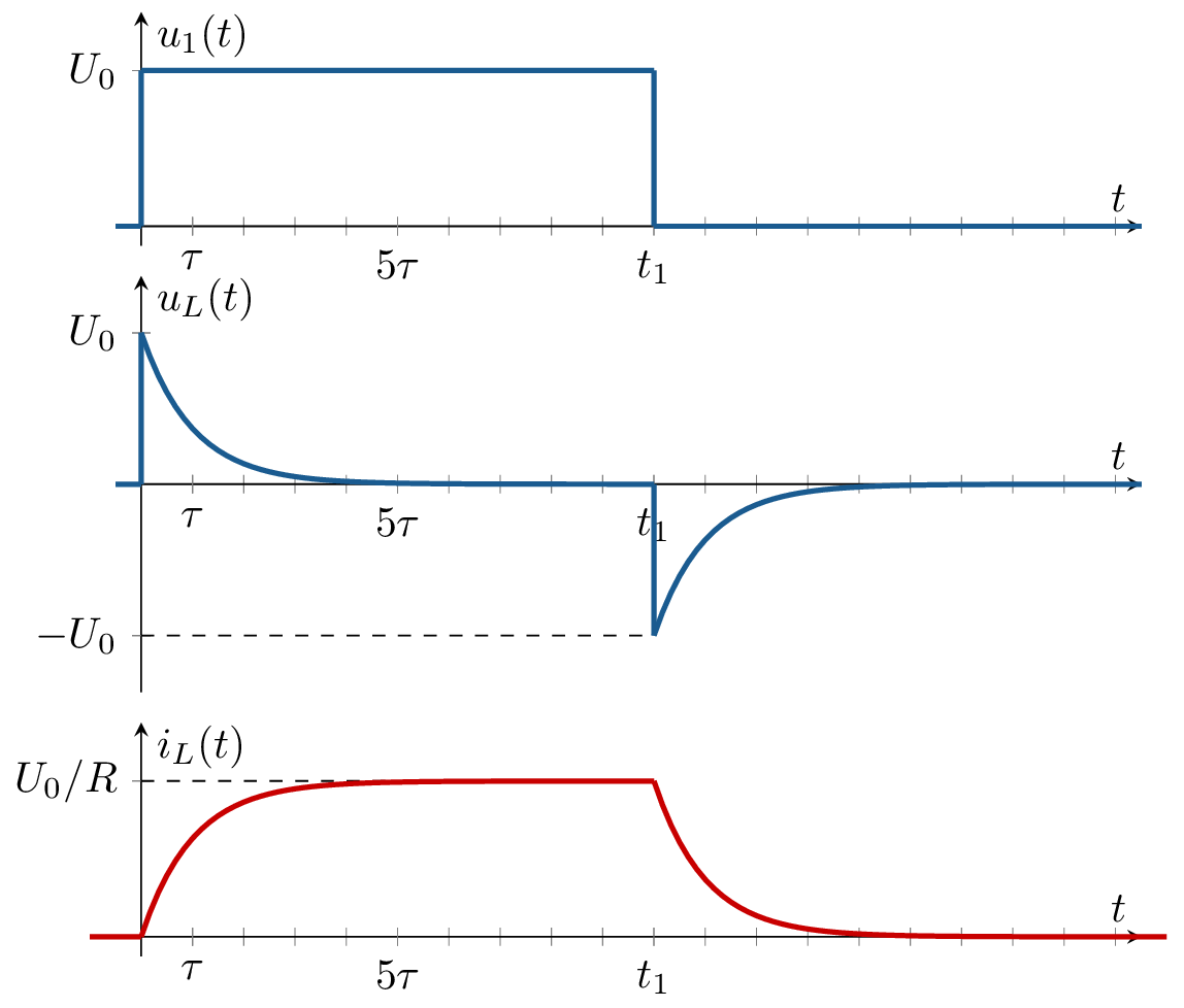
e) Temporal progression of \(u_L, i_L, u_R\).
The switch-on behavior of a series circuit consisting of a resistive resistor \(R\) and an inductance \(L=100\,\text {mH}\) is to be
examined. At time \(t=0\), a voltage \(u=U_0 = 35\,\text {V}\) is applied to the series circuit. For \(t \leq 0\), \(u=0\). The inductor voltage at time \(t_1=3\,\text {ms}\) is known
and amounts to \(u_L(t_1)=26\,\text {V}\).
Determine the time constant \(\tau \), the resistance \(R\), and the voltage \(u_R(t=5\,\text {ms})\).
\begin {align*} \text {ODE:}&& \frac {L}{R}\cdot \mathrm{d}t i+i&=\frac {U_0}{R}\\ \text {Solution:}&&i&=\frac {U_0}{R}\cdot (1-e^{-\frac {t}{\tau }}) \text {with} \tau = \frac {L}{R} \end {align*}
\begin {align*} u_L &= L\cdot \mathrm{d}t i =U_0\cdot e^{-\frac {t}{\tau }}\\ u_R &= u-u_L = U_0\cdot (1-e^{-\frac {t}{\tau }})\\ i(t=3\,ms)&= \frac {U_0}{R}\cdot (1-e^{-\frac {t}{\tau }})\\ u_L(t=3\,ms)&= U_0\cdot e^{-\frac {t}{\tau }} = 26\,V\\ \frac {u_L(t=3\,ms)}{U_0}&=e^{-\frac {t}{\tau }}\\ -\frac {t}{\tau }&=\ln \left (\frac {u_L(t=3ms)}{U_0}\right )\\ \tau &=-\frac {t}{\ln \left (\frac {u_L(t=3ms)}{U_0}\right )} = -\frac {3ms}{\ln \left (\frac {26\,V}{35\,V}\right )} = 10,1\,ms\\ R &= \frac {L}{\tau } = \frac {100\,mH}{10,1\,ms} = 9,9\,\Omega \\ u_R(t=5\,ms)&=U_0\cdot (1-e^\frac {-5\,ms}{10,1\,ms})\\ &=35\,V\cdot 0,39 = 13,65\,V \end {align*}
The switch in the circuit shown on the right is closed at time
\(t=0\).
| \(R_1 = 1{,}2\,\text k \Omega \) | \(R_2 = 2\,\text k \Omega \) | |
| \(C_1 = 1\,\mu \text F\) | \(R_3 = 500\,\Omega \) | |
| \(U_q = 250\,\text {V}\) |
Determine the time course of the current \(i_3\) through the
resistor \(R_3\) and plot it as a function of time (line graph) for \(-\tau <t<5\tau \).
The network is in a steady state at time \(-\tau \). Here, \(\tau \) is the time constant of the network.
Set up the ODE for \(u_C\) and determine the current \(i_3\) via \(i_3=\frac {u_C}{R_3}\).
Combine \(R_1\) and \(R_2\) as a parallel connection \(R_{12}\) after the switching instant (\(t>0\)).
1st ODE for \(u_C\) (\(t > 0\)) with \(i_3=\frac {u_C}{R_3}\): \begin {align*} U_q &= u_{12} + u_C &&\text {with} u_{12} {\text { via parallel connection of $R_1$ and $R_2$}}\\ &= R_{12} \cdot i_{12} + u_C &&\text {with} R_{12}=R_1||R_2,& i_{12}&=i_C+i_3\\ &= R_{12} \cdot (i_C + i_3) + u_C &&\text {with} i_{C}=C\cdot \mathrm{d}t \,u_C,& i_3&=\frac {u_C}{{R_3}}\\ &= R_{12} \cdot (C \cdot \mathrm{d}t \,u_C + \frac {u_C}{{R_3}}) + u_C\\ &= C \cdot R_{12} \cdot \mathrm{d}t \,u_C + \left ( \frac {R_{12}}{{R_3}} + 1 \right ) \cdot u_C& &\bigg |\ \cdot R_3\\ U_q \cdot R_3 &= C \cdot R_{12} \cdot R_3 \cdot \mathrm{d}t \,u_C + \left (R_{12}+R_3\right ) \cdot u_C& &\bigg | :\left (R_{12}+R_3\right )\\ U_q \cdot \frac {R_3}{R_{12}+R_3} &= \underbrace {C \cdot \frac {R_{12} \cdot R_3}{R_{12} + R_3}}_{\tau } \cdot \mathrm{d}t \,u_C + u_C& &\Longrightarrow \tau =C \cdot \frac {R_{12} \cdot R_3}{R_{12} + R_3} \end {align*}
3. Homogeneous solution (fleeting) and 2. Particular solution (\(t \to \infty \), settled in): \begin {align*} u_{C,\mathrm {h}} &= K \cdot \mathrm {e}^{-\frac {t}{\tau }}& &\text {with} \tau =C \cdot \frac {R_{12} \cdot R_3}{R_{12} + R_3} \\ u_{C,\mathrm {p}} &= U_q \cdot \frac {R_3}{R_{12}+R_3}& &\text {$C_1$ corresponds to idle} \end {align*}
4. superposition and 5. Determine constant(s): \begin {align*} u_C &= u_{C,\mathrm {h}} + u_{C,\mathrm {p}}\\ u_C(t=0) &= K \cdot \cancel {\mathrm {e}^{0}} + U_q \cdot \frac {R_3}{R_{12}+R_3} \overset {!}{=} U_q& &\text {(Initial condition)}\\ \Rightarrow K &= U_q \cdot \left ( 1 - \frac {R_3}{R_{12}+R_3} \right )\\ &= U_q \cdot \frac {R_{12}}{R_{12}+R_3}\\[2pt] u_C &= U_q \cdot \left ( 1 - \frac {R_3}{R_{12}+R_3} \right ) \cdot \mathrm {e}^{-\frac {t}{\tau }} + U_q \cdot \frac {R_3}{R_{12}+R_3}& &\bigg | :R_3\\[2pt] i_3 &= U_q \cdot \left ( \frac {1}{R_3} - \frac {1}{R_{12}+R_3} \right ) \cdot \mathrm {e}^{-\frac {t}{\tau }} + U_q \cdot \frac {1}{R_{12}+R_3} \end {align*}
Time constant \(\tau \) and initial and final values of the current \(i_3\) for sketch:
At time \(t=t_0\), the alternating voltage \(u_1(t)\) is applied to the entire circuit consisting of \(R_1\) in series with the parallel connection of \(R_2\) and \(C\). For \(t<t_0\), the circuit is in a steady state. The source voltage is given by \(u_1(t) = \hat {U}_1 \cdot \sin (\omega t)\).

Time points for minimum and maximum volatile state (\(t_{min},\ t_{max}\)).
No settling if \(i_{L,f}=0 \Leftrightarrow i_L=i_{L,e} \Leftrightarrow i_L(t_0)=i_{L,e}(t_0)\) applies.
That is, for a vanishing transient state (no settling process), the following applies: \begin {align*} &\text {IC:}&i_L(t_0) = i_{L,e}(t_0) &= \hat {I_{L,e}} \cdot \sin (\omega t_0 + \varphi ) \overset {!}= 0 & &\Rightarrow i_L(t')=i_{L,e}(t') \Leftrightarrow i_{L,f}(t')=0\\ &&\Leftrightarrow \omega t_0 + \varphi &\overset {!}{=} 0 + n\cdot \pi & &\text {with} n \in \mathbb {N} \\ &&t_{min} &= \frac {n\cdot \pi - \varphi }{\omega } & &\text {corresponds to zero crossings of $i_{L,e}$}\\ \end {align*}
And for maximum transient state (switching point offset by \(90^\circ \)), the following applies: \begin {align*} &&t_{max} &= \frac {n\cdot \pi - \varphi }{\omega } + \frac {T}{4} & &\text {corresponds to extreme points of $i_{L,e}$} \end {align*}
Maximum current during the transient process sought. Switching time \(t_0\) at negative peak value of \(i_{L,e}\). Let \(t' = t - t_0\), i.e. \(t'=0\) at the switching time, then the following applies: \begin {align*} i_L(t') &= i_{L,h}(t') + i_{L,e}(t') \\ &= K \cdot \mathrm {e}^{-\frac {t'}{\tau }} - \hat {I_{L,e}} \cdot \cos (\omega t')\\ \text {AB:} i_L(t'=0) &= K - \hat {I_{L,e}} \overset {!}{=}0 \Rightarrow K = \hat {I_{L,e}}\\ i_L(t') &= \hat {I_{L,e}} \cdot \left ( \mathrm {e}^{-\frac {t'}{\tau }} - \cos (\omega t') \right ) \\ \end {align*}
Maximum at positive peak value (\(180^\circ \) to \(t_0\)): \begin {align*} i_{L,max} &= i_L(t' = \frac {\pi }{\omega }) \\ &= \hat {I_{L,e}} \cdot \left ( \mathrm {e}^{-\frac {T/2}{T}} - \cos (\pi ) \right ) \\ &= \hat {I_{L,e}} \cdot \left ( \mathrm {e}^{-\frac {1}{2}} + 1\right ) = 1,606 \cdot \hat {I_{L,e}} \end {align*}

Aufgaben
Introduction to switching operations...