The electric current

1 The electric flow field

The previous chapters refer exclusively to stationary charge carriers. Consequently, this subfield of electrical engineering is referred to as electrostatics.

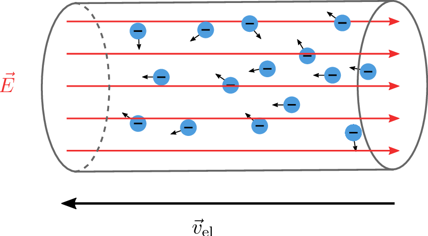
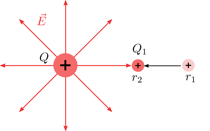
At the molecular level, the free electrons in an electrical conductor constantly move in random directions. On average, however, the movement of the individual electrons balances out. If an electric field \(\vec {E}\) is applied to a conductor, the free moving electrons in it are attracted towards the positively charged electrode (see Figure 1) . In addition to the random, undirected motion, a directed motion component is added. If such a directed motion of particles occurs, it is referred to as a flow field.

In addition to electrons in conductors, an electric flow field can also be caused by charged ions in gases or liquids. In the case of a charge carrier movement that is constant on average over time, which is achieved in the conductor shown by a constant electric field, a stationary electric flow field is present.

2 Electric current

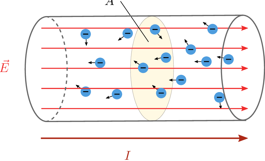
Electrical current \(I\) refers to the directed movement (drift movement) of electrical charge carriers. The direction of the electric current is defined as running from the higher potential (positively charged electrode) to the lower potential. It therefore runs in the same direction as the electric field strength, but in the opposite direction to the drift velocity of the electrons (see Figure 2).

The electrons reach a field strength-dependent drift velocity \(\vec {v}_\mathrm {el}\). Collisions with the metal atoms from the lattice structure impede the free movement of the electrons and counteract it as a kind of resistance.

\begin {equation} \vec {v}_\mathrm {el} = - b_\mathrm {el} \cdot \vec {E} \label {eq:driftgeschw} \end {equation}

\begin {equation*} [ \vec {v}_\mathrm {el} ] = \frac {\mathrm {m}}{\mathrm {s}} \end {equation*}

The proportionality factor \(b_\mathrm {el}\) between the drift velocity \(\vec {v}_\mathrm {el}\) and the electric field strength \(\vec {E}\) is referred to as electron mobility.

\begin {equation*} [b_\mathrm {el}] = \frac {\mathrm {m}^2}{\mathrm {Vs}} \end {equation*}

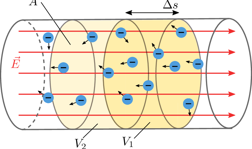
In addition to the drift velocity \(\vec {v}_\mathrm {el}\), the number of electrons \(N_\mathrm {el}\) and their charge quantity \(\Delta Q\) are also relevant for determining the electric current \(I\).

The charge quantity \(\Delta Q\) corresponds to

\begin {equation*} \Delta Q = e \cdot N_\mathrm {el} = e \cdot n_\mathrm {el} \cdot V_1 \, \end {equation*}

where \(n_\mathrm {el}\) indicates the density of charge carriers in volume \(V_1\).

With \(V_1 = \Delta s \cdot A\) and \(\Delta s = v_\mathrm {el} \cdot \Delta t\), we get:

\begin {equation*} \Delta Q = e \cdot n_\mathrm {el} \cdot v_\mathrm {el} \cdot \Delta t \cdot A \end {equation*}

Using the definition of drift velocity (1), this leads to:

\begin {equation*} \Delta Q = e \cdot n_\mathrm {el} \cdot b_\mathrm {el} \cdot E \cdot \Delta t \cdot A \, , \end {equation*}

from which the change in charge quantity \(\Delta Q\) per unit of time \(\Delta t\) can be derived:

\begin {equation*} \frac {\Delta Q}{\Delta t} = e \cdot n_\mathrm {el} \cdot b_\mathrm {el} \cdot E \cdot A \end {equation*}

3 Definition of electrical current

The change in charge over time determined in this way is referred to as electric current \(I\):

\begin {equation} I = \frac {\Delta Q}{\Delta t} \label {eq:stromdef} \end {equation}

\begin {equation*} [I] = \mathrm {Ampere} = \mathrm {A} \end {equation*}

From this definition of current, it follows that the electrical current accumulated over a period of time results in the amount of charge \(Q\) transported during that time.:

\begin {equation} Q = \int _{t_1}^{t_2} i(t) \, \mathrm {d} t \end {equation}

In addition to the total electric current \(I\), the current relative to the conductor cross-section is often also of interest. To calculate this current density \(J\), the current \(\Delta I\) is considered through an elementary small area element \(\Delta A\):

\begin {equation} J = \frac {\Delta I}{\Delta A} \end {equation}

If the electric current \(I\) is evenly distributed across a surface, this can be simplified:

\begin {equation} J = \frac {I}{A} \end {equation}

Since the current \(I\) remains identical across the entire conductor, a reduction in the cross-sectional area of the conductor also changes the resulting electric current density \(J\) (see Figure 4).

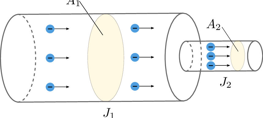
The following applies here:

\begin {equation*} J_1 \cdot A_1 = J_2 \cdot A_2 = I \end {equation*}

A current of \(I = 8 \mathrm {A}\) flows through a copper wire with a cross-sectional area of \(A = 1 \mathrm {mm}^2\). One \(\mathrm {mm}^3\) contains approximately \( 8.5 \cdot 10^{19}\) atoms. Let us assume that 1 electron per atom is involved in charge transport.

What is the average drift velocity of the electrons through the wire?

\begin {equation*} \vec {v}_\mathrm {el} = - b_\mathrm {el} \cdot \vec {E} \end {equation*}

Since the negatively charged electrons move in the opposite direction to the field direction \(\vec {E}\) (and thus also in the opposite direction to the technical current direction \(I\)), the direction of the drift velocity is sufficiently described, and it is sufficient to calculate the magnitude \(v_\mathrm {el}\).

With the connection

\begin {equation*} I = e \cdot n_\mathrm {el} \cdot b_\mathrm {el} \cdot E \cdot A\\ \rightarrow E = \frac {I}{e \cdot n_\mathrm {el} \cdot b_\mathrm {el} \cdot A} \end {equation*}

results in:

\begin {equation*} v_\mathrm {el} = \cancel {b_\mathrm {el}} \cdot \frac {I}{e \cdot n_\mathrm {el} \cdot \cancel {b_\mathrm {el}} \cdot A} \end {equation*}

Inserting the numerical values:

\begin {equation*} v_\mathrm {el} = \frac {8 \mathrm {A}}{1,602 \cdot 10^{-19} \, \mathrm {As} \cdot 8,5 \cdot 10^{19} \, \mathrm {mm}^{-3} \cdot 1 \, \mathrm {mm}^2 } \end {equation*}

\begin {equation*} v_\mathrm {el} = 0,59 \frac {\mathrm {mm}}{s} \end {equation*}

The electrons therefore move at an average speed of 0.59 mm/s. However, since the electric field strength within the conductor travels at the speed of light, all the electrons in the conductor start moving at practically the same time. This can be compared to a tube completely filled with marbles. The moment another marble is pushed in, a marble falls out on the other side, even though the individual marbles are moving slowly.