Fundamentals of Complex Numbers
The phasor diagrams used in alternating current technology provide a quick overview of the magnitude and direction of the voltage and current. The underlying concepts of the complex number plane and the structure of phasor diagrams are explained in more detail below and illustrated with an example.
Learning objectives: Complex numbers
The Students can
- handle numbers in the complex plane.
- Plot phasor diagrams of complex numbers.
- calculate complex numbers.
1 Complex number plane
In order to understand the structure of pointer diagrams, a basic understanding of the complex number system is necessary. For elementary arithmetic operations, natural numbers including zero and rational numbers are sufficient. Rational numbers can be represented as finite or periodic decimal numbers. Irrational numbers, on the other hand, can be represented as decimal numbers that have an infinite number of digits and are not periodic. Real numbers are composed of rational numbers and irrational numbers. However, it is not possible to take the square root of a negative number in the real number system. For this purpose, the complex number system is introduced. In the complex number system, the real number space is extended by the imaginary unit j. Thus, in the complex number system, taking the square root of -1 results in the imaginary unit j.
\begin {equation} \mathrm {j}=\sqrt {-1} \end {equation}
Squaring the imaginary unit again gives -1.
\begin {equation} \mathrm {j}^2=-1 \end {equation}
A complex number Z describes a location in the complex plane. To uniquely define a location in a two-dimensional coordinate system, two coordinates are required. The two coordinates for describing a complex number Z are described in the complex plane as the real part and the imaginary part (see Equation 3). Complex numbers are usually indicated by an underscore, whereby the real part and the imaginary part represent real numbers.
\begin {equation} \underline {Z}=Real part+\mathrm {j} \cdot Imaginary\ part \label {GleichungKomplexeZahlen} \end {equation}
\begin {equation} \underline {Z}=\Re (\underline {Z})+\mathrm {j} \cdot \Im (\underline {Z}) \end {equation}
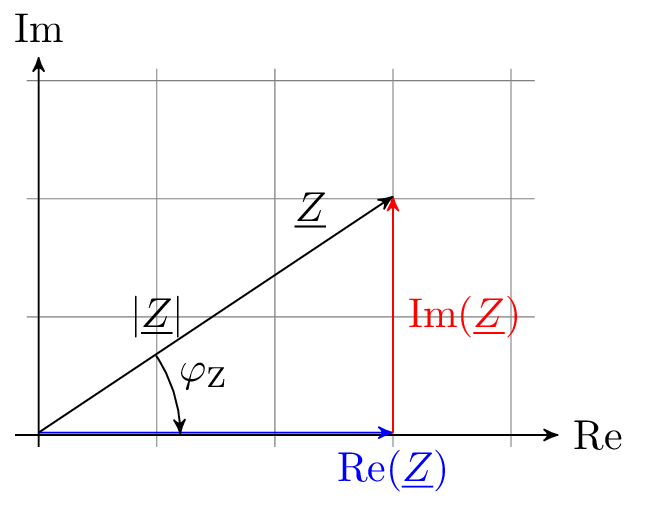
In the complex plane, the real part is plotted on the abscissa and the imaginary part on the ordinate. The abbreviations Re = real part and Im = imaginary part are used. The coordinate system of a complex plane is explained in Figure 1. The location of the complex number can be represented by direction arrows, also known as vectors or pointers. The representation of the complex number in Cartesian coordinates is achieved by decomposing it into the real part of the complex number Re(Z) and the imaginary part of the complex number Im(Z) combined with the imaginary unit j. Complex numbers can also be represented in polar coordinates. This is done by the magnitude \(|\underline {Z}|\) of the complex number Z and by the angle \(\varphi \) that the pointer of the complex number encloses with the real axis.
The two forms of representation can be transformed into each other. Euler’s formula is helpful here. Euler’s formula shows that the ordinate value and the abscissa value of the unit circle can be calculated using the trigonometric functions cosine and sine. Euler’s formula is represented in equation 5.
\begin {equation} \mathrm {e}^{\mathrm {j} \cdot \chi } = \cos (\chi ) + \mathrm {j} \cdot \sin (\chi ) \label {GleichungEuler} \end {equation}
Using Euler’s formula, the polar coordinates can be transformed into Cartesian coordinates by adding the absolute value of the complex number. This is explained by equation 6.
\begin {equation} \underline {Z} = |\underline {Z}| \cdot \cos (\varphi ) + \mathrm {j} \cdot |\underline {Z}| \cdot \sin (\varphi ) = \Re (\underline {Z}) + \mathrm {j} \cdot \Im (\underline {Z}) \label {GleichungKartesisch} \end {equation}
Using Pythagoras’ theorem, the real and imaginary parts of the complex number can be used to determine the magnitude of the complex number for the polar coordinates. The corresponding angle is obtained from the arctan with the ratio of the imaginary part to the real part in the argument. With this information, a complex number such as in equation 7 can be transformed into polar coordinates.
\begin {equation} \underline {Z} = \sqrt {(\Re (\underline {Z}))^2+(\Im (\underline {Z}))^2} \cdot \mathrm {e}^{\mathrm {j} \cdot \arctan (\frac {\Im (\underline {Z})}{\Re (\underline {Z})}) } = |\underline {Z}| \cdot \mathrm {e}^{\mathrm {j} \cdot \varphi } \label {GleichungPolar} \end {equation}
Key point: Representations of complex numbers
Cartesian representation: \begin {equation} \underline {Z} = \Re (\underline {Z}) + j \cdot \Im (\underline {Z}) \nonumber \end {equation} Polar form: \begin {equation} \underline {Z} = |\underline {Z}| \cdot e^{j \cdot \varphi } \nonumber \end {equation} Trigonometric representation: \begin {equation} \underline {Z} = |\underline {Z}| (\cos (\varphi ) + j \cdot \sin (\varphi )) \nonumber \end {equation}
Conjugation is one of the operations on complex numbers. When conjugating a complex number, the j is replaced by -j (negation of the imaginary part). As shown in Equation 11, conjugation is indicated by an asterisk.
\begin {equation} \underline {Z}^* = (\Re (\underline {Z}) + \mathrm {j} \cdot \Im (\underline {Z}))^*= \Re (\underline {Z}) - \mathrm {j} \cdot \Im (\underline {Z}) \label {GleichungKonj} \end {equation}
The magnitude of a complex number can be determined by multiplying the complex number by its conjugate (see Equation 12). Instead of the magnitude, which contains a root, the square of the magnitude is also used. It also represents a measure of the distance of the number from the origin, but is easier to calculate.
\begin {equation} |\underline {Z}| = \sqrt {\underline {Z} \cdot \underline {Z}^*} \rightarrow |\underline {Z}|^2 = \underline {Z} \cdot \underline {Z}^* \label {GleichungBetrag} \end {equation}
When adding and subtracting complex numbers, it is advisable to first convert them into Cartesian coordinates. This allows the real part and the imaginary part of the complex number to be calculated separately. \begin {align} \underline {Z}_1+\underline {Z}_2 = \Re (\underline {Z}_1) + \Re (\underline {Z}_2) +j \cdot (\Im (\underline {Z}_1) + \Im (\underline {Z}_2)) \\ \underline {Z}_1-\underline {Z}_2 = \Re (\underline {Z}_1) - \Re (\underline {Z}_2) -j \cdot (\Im (\underline {Z}_1) - \Im (\underline {Z}_2)) \end {align}
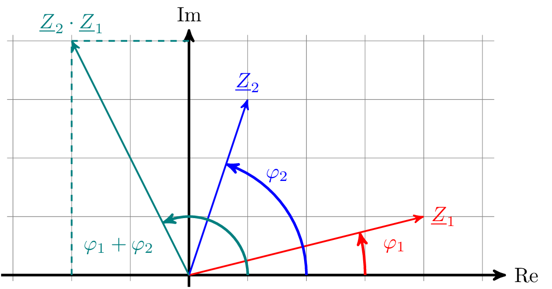
The representation in polar coordinates is recommended for calculating complex numbers by multiplication and division. The multiplication of complex numbers is composed of the product of the magnitudes and the sum of the respective angles (see Equation 13). In division, the magnitudes are divided and the angles are subtracted from each other (see Equation 14).
\begin {equation} \underline {Z}_1 \cdot \underline {Z}_2 = |\underline {Z}_1| \cdot |\underline {Z}_2| \cdot e^{j \cdot (\varphi _1+\varphi _2)} \label {GleichungMultiplikation} \end {equation}
\begin {equation} \frac {\underline {Z}_1}{\underline {Z}_2} = \frac {|\underline {Z}_1|}{|\underline {Z}_2|} \cdot e^{j \cdot (\varphi _1-\varphi _2)} \label {GleichungDivision} \end {equation}
Key point: Basic arithmetic operations with complex numbers
For addition and subtraction, the Cartesian representation is generally used for complex numbers. For multiplication and division of complex numbers, the polar form is chosen.
Since the division is initially only defined for real numbers other than zero, the complex number in the denominator is extended so that it becomes real. \begin {equation} \frac {\underline {Z}_1}{\underline {Z}_2} = \frac {\underline {Z}_1}{\underline {Z}_2} \cdot \frac {\underline {Z}_2^*}{\underline {Z}_2^*} = \frac {\underline {Z}_1 \cdot \underline {Z}_2^*}{|\underline {Z}_2|^*} \end {equation}
Adding a complex number to its conjugate cancels out its imaginary part (see equation 16). Similarly, subtracting the real part cancels it out (see equation 17).
\begin {equation} \Re (\underline {Z}) = \frac {\underline {Z}+\underline {Z}^*}{2} \label {GleichungRealteil} \end {equation} \begin {equation} \Im (\underline {Z}) = \frac {\underline {Z}-\underline {Z}^*}{2j} \label {GleichungImaginärteil} \end {equation}
2 Graphical representation and calculations with complex numbers
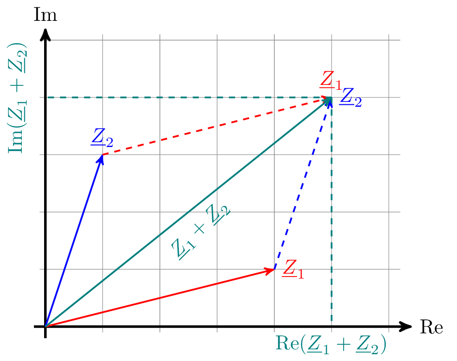
Complex numbers can also be solved graphically using pointer diagrams. If the complex numbers are represented in Cartesian form as recommended, the components of the real parts and the imaginary parts can be read directly and entered into a coordinate system. The complex numbers are entered, for example, in Figure 2. When adding complex numbers, either \(Z_\mathrm {1}\) is set to \(Z_\mathrm {2}\) or vice versa. This is because the commutative law still applies to addition. Here, the dashed arrows indicate the parallel shifts of \(Z_\mathrm {1}\) and \(Z_\mathrm {2}\). Both shifts end at the same coordinate. Here, the real part and the imaginary part can be read separately from the sum of the two complex numbers.
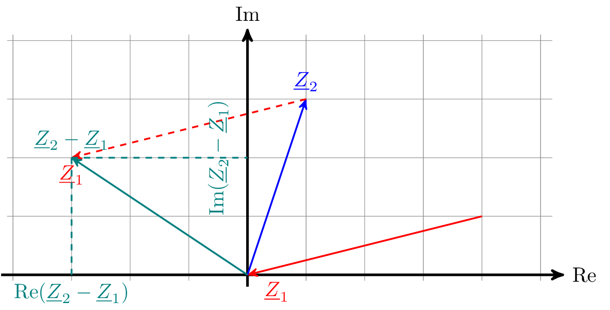
The graphical solution for subtracting complex numbers is similar to that for addition. It should be noted that, as in other number systems, the commutative law does not apply when subtracting two complex numbers. If the complex number \(Z_\mathrm {2}\) is subtracted from \(Z_\mathrm {1}\), the direction of \(Z_\mathrm {1}\) changes. Here, the parallel shift occurs again, but only for \(Z_\mathrm {1}\). The resulting new vector can then be read again as the real part and the imaginary part.
The complex numbers \(\underline {Z}_\mathrm {1}\) and \(\underline {Z}_\mathrm {2}\) shown in Figure 4 are represented for multiplication in polar coordinates. Using the previously described calculation rules for multiplication of complex numbers, the values for the result \(\underline {Z}_\mathrm {3}\) can be determined. The multiplication of the pointer lengths gives the length of the product. The sum of the two complex numbers gives the angle of the new complex number.