Complex alternating current calculation

Direct current networks use constant voltage sources and current sources. In contrast, complex alternating current calculations use sources with sinusoidal alternating quantities. The electrical analysis of components in an alternating voltage network is complex. The complex voltages U and currents I generate time-dependent voltage values u(t) and current values i(t). Equation 1 describes the specified relationship between complex and time-dependent current and voltage values for an ohmic resistor.

Complex and time-dependent current and voltage specifications in AC calculation:

\begin {equation} \underline {U} = \underline {Z}_\mathrm {R} \cdot \underline {I} \rightarrow u(t) = R \cdot i(t) \label {GleichungURIKomplex} \end {equation}

Apart from the complexity of alternating current calculations, the rules for calculating electrical networks still apply, such as mesh and node rules, the behaviour of series and parallel circuits, node potential analysis, and mesh current analysis. In all these examples, care must be taken to calculate with complex alternating quantities. For the explanation of electrical networks with complex alternating quantities, the following topics are examined in more detail below: For the calculation of electrical networks with alternating quantities, the following topics are examined in more detail below:

1 Impedance and admittance in the complex plane

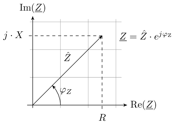
A phase shift between the voltage and the current results in the generation of a reactive component of the impedance. However, the reactive component cannot be represented on the real axis, which is why the real axis is extended by an imaginary axis, which together form the complex plane. Figure 1 shows the phasor of the complex impedance in the complex plane with imaginary and real components.

According to equation 2, the complex impedance Z also consists of a real part and an imaginary part. The real part consists of the ohmic component, which represents the effective resistance of an impedance. The effective resistance is also referred to as resistance R. The second component of impedance is the imaginary part, which is also referred to as reactance X. The reactance of an electrical network, for example, consists of the capacitive and inductive effects and is assigned the imaginary unit j. As in direct current technology, the unit of complex impedance is the ohm \(\Omega \).

\begin {equation} Impedance = Resistance + j \cdot Reactance \rightarrow \underline {Z} = R + j \cdot X \label {GleichungImpedanz} \end {equation} \begin {equation} [\underline {Z}] = 1\ Ohm = 1\ \Omega \nonumber \end {equation}

As in direct current technology, there is a conductance value for electrical resistance in complex alternating current technology. This reciprocal value of the complex impedance is referred to as admittance Y (see equation 4). The unit of the complex conductance remains Siemens S, as in direct current technology.

\begin {equation} R = \frac {1}{G} \rightarrow \underline {Z} = \frac {1}{\underline {Y}} \label {GleichungImpedanzAttmitanz} \end {equation}

Admittance can also be differentiated into a real conductance and a reactive conductance. The real conductance G of the admittance is referred to as conductance, and the reactive conductance B of the admittance is referred to as susceptance (see Equation 5 ).

\begin {equation} Admittance = Conductance + j \cdot Susceptibility \rightarrow \underline {Y} = G + j \cdot B \label {GleichungAdmittanz} \end {equation}

\begin {equation} [\underline {Y}] = 1\ Siemens = 1\ S \nonumber \end {equation}

2 Complex resistance

The complex resistance of an ohmic consumer consists of the active component R and the reactive component of the ohmic resistance. The ohmic resistance R embodies the property of conductive materials to convert electrical power into thermal power. The reactive component of the resistance does not convert the power of alternating currents into heat. The reactive component of the electrical resistance is denoted as \(X_\mathrm {R}\). However, since the ideal electrical resistance is purely resistive and therefore purely real, the symbol R is often used. Equation 7 explains these relationships.

\begin {equation} \underline {Z}_\mathrm {R} = R + j \cdot X_\mathrm {R} { \rightarrow X_\mathrm {R-ideal} = j \cdot 0\ \Omega } { \rightarrow \underline {Z}_\mathrm {R} = R} \label {GleichungWid1} \end {equation}

The time-dependent values for voltage and current result in the relationships of ideal ohmic resistance according to equation 8.

\begin {equation} \underline {U} = \underline {Z}_\mathrm {R} \cdot \underline {I} \rightarrow u(t) = R \cdot i(t) \label {GleichungWid2} \end {equation}

An ideal electrical resistance is a pure active resistance and has no reactive resistance components. Real electrical resistance is subject to parasitic effects. The circuit diagrams of an ideal and a real electrical resistance are compared in Figure 2. These parasitic effects have an inductive effect, illustrated by the coil, and a capacitive effect, illustrated by the capacitance, on the circuit. In addition to the frequency dependence of the parasitic effects, the voltage and current are also divided in such a way that the entire power no longer drops across the resistor. The impedance of the ideal electrical resistor is not frequency-dependent.

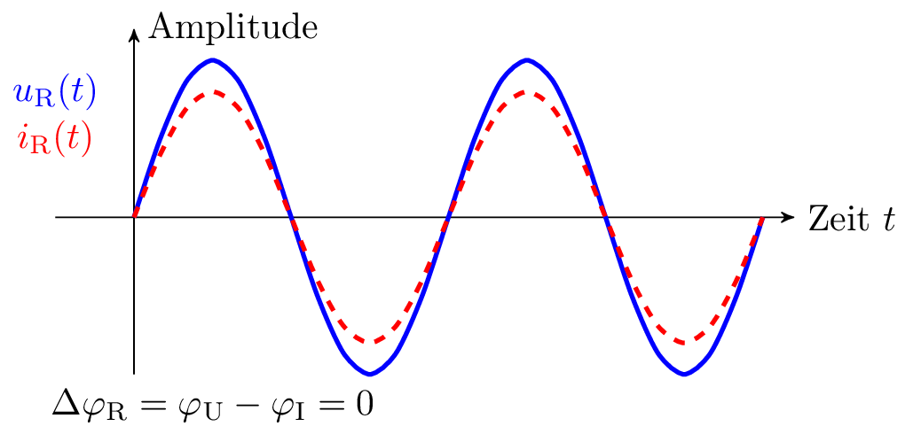
With ideal electrical resistance, there is no phase shift between the voltage and the current. In Figure 3, the sine waves for the voltage and current are plotted on an ideal resistor. They lie on top of each other without any phase shift, meaning they are in phase.

3 Capacity

As a component in electrical engineering, the capacitor has the ability to store energy between the two plates in the electric field. The size of a capacitor is specified in terms of its capacitance C. The unit of capacitance is the farad F. The complex impedance of a capacitor can be calculated using equation 9. In contrast to the ideal resistor, the ideal capacitor in an alternating current circuit does not act solely as an effective resistance. The real capacitor acts both through an effective component and through an reactive component. The circular frequency \(\omega \) is frequency-dependent. This results in low impedance values for the capacitor at high frequencies. Conversely, high impedance values result at low frequencies. The reactive component of the capacitor acts as capacitive reactance. The capacitor can also be calculated using complex admittance. The complex admittance is derived from the reciprocal of the complex impedance of the capacitor.

\begin {equation} \underline {Z}_\mathrm {C} = \frac {1}{j \omega C} \rightarrow \underline {Y}_\mathrm {C} = j \omega C \label {GleichungKap1} \end {equation}

The ideal capacitor acts purely in the reactive component, so according to equation 10 from the complex notation \(Z_C\), the reactive component of the capacitor \(X_C\) with time-dependent voltage and current.

\begin {equation} \underline {U} = \underline {Z}_\mathrm {C} \cdot \underline {I} \qquad \qquad u(t) = \underline {X}_\mathrm {C} \cdot i(t) \label {GleichungKap2} \end {equation}

It is assumed that the alternating voltage at a capacitor has a phase shift of 0°. With this assumption, the phase shift of the current at the capacitor can be determined using equation 11. Due to the phase shift of the current, the curve of a cosine function contrasts with the sine function of the voltage. If both the voltage and the current are to be described by the sine function, the phase shift \(\Delta \varphi \) of \(\pi /2\) is included in the argument.

\begin {equation} u(t) = \hat {U} \cdot \sin (\omega t) \qquad i(t) = \hat {I} \cdot \cos (\omega t) = \hat {I} \cdot \sin (\omega t + \pi /2) \label {GleichungKap3} \end {equation}

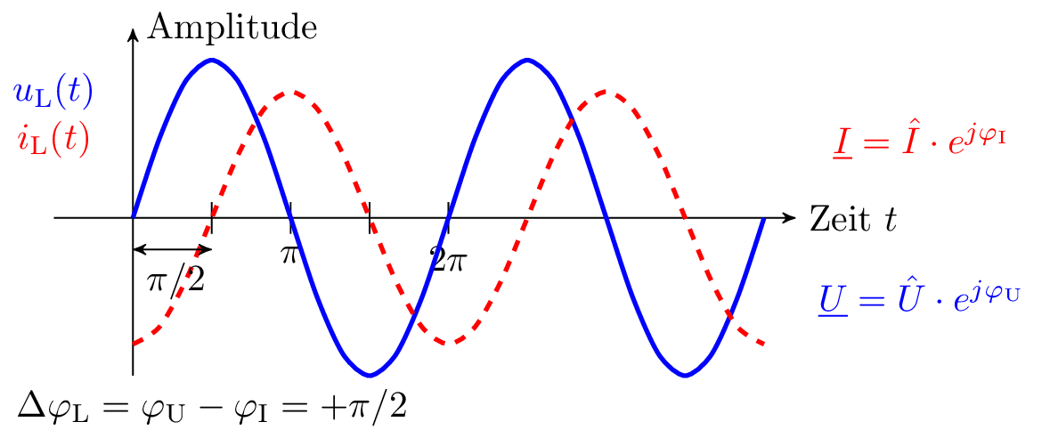
With inductors and capacitors, there is a phase shift between the alternating voltage and the alternating current. With capacitors, this means that the current leads the voltage by 90° (degrees). The described phenomenon of phase shift is illustrated in Figure 4. The current shown in red at a capacitor reaches its maximum value \(2\pi \) (radians) earlier than the blue-coloured maximum value of the voltage.

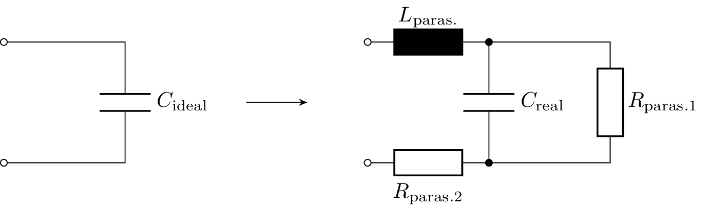
As a rule, calculations are based on ideal components and their properties. However, real capacitors, like the real resistors described above, exhibit inductive and ohmic parasitic effects. The ideal capacitor is compared with the real capacitor in Figure 5. The input and output lines exhibit inductive (\(L_\mathrm {paras.}\)) and ohmic (\(R_\mathrm {paras.2}\)) components. In addition, the capacitor is subject to constant self-discharge. This self-discharge occurs symbolically via the parallel resistance \(R_\mathrm {paras.1}\).

4 Inductance

The coil is also an energy storage device, just like the capacitor. However, in the case of the coil, the energy is not stored in an electric field, but in a magnetic field according to the laws of induction. The size of a coil is given by its inductance L. The unit of inductance is Henry H. The complex impedance of a coil is given by the imaginary unit j, the angular frequency \(\omega \) and the inductance L (see Equation 12). The complex admittance is calculated by the reciprocal of the coil impedance. This leads to relationships that develop contrary to the impedance calculations for capacitances. At high frequencies, the impedances of coils also become large in accordance with their inductance and correspondingly small at low frequencies.

\begin {equation} \underline {Z}_\mathrm {L} = j \omega L \rightarrow \underline {Y}_\mathrm {L} = \frac {1}{j \omega L} \label {GleichungInd1} \end {equation}

As with the capacitor, the ideal coil acts purely as a reactive component of the impedance. In equation 13, the complex notation of the coil impedance \(Z_L\) is used on the left-hand side. On the right-hand side, the time function is represented solely by the notation of the reactive component of the coil \(X_L\).

\begin {equation} \underline {U} = \underline {Z}_\mathrm {L} \cdot \underline {I} \qquad \qquad u(t) = \underline {X}_\mathrm {L} \cdot i(t) \label {GleichungInd2} \end {equation}

In principle, the time functions of inductances for voltage and current behave similarly to the time functions of capacitances. Only the phase shift of the current in coils is opposite to the phase shift of capacitors. The phase shift \(\Delta \varphi \) between the voltage and the current at an inductance is \(\pi /2\).

\begin {equation} u(t) = \hat {U} \cdot \cos (\omega t) = \hat {U} \cdot \sin (\omega t + \pi /2) \qquad i(t) = \hat {I} \cdot \sin (\omega t) \label {GleichungInd3} \end {equation}

Equivalent to the phase shift at a capacitor, there is also a phase shift at the inductance. However, this phase shift of the current at the inductance is opposite to the phase shift of the capacitance. In the specific case shown in Figure 6, it can be seen that the current (red) at an inductance lags behind the voltage (blue).

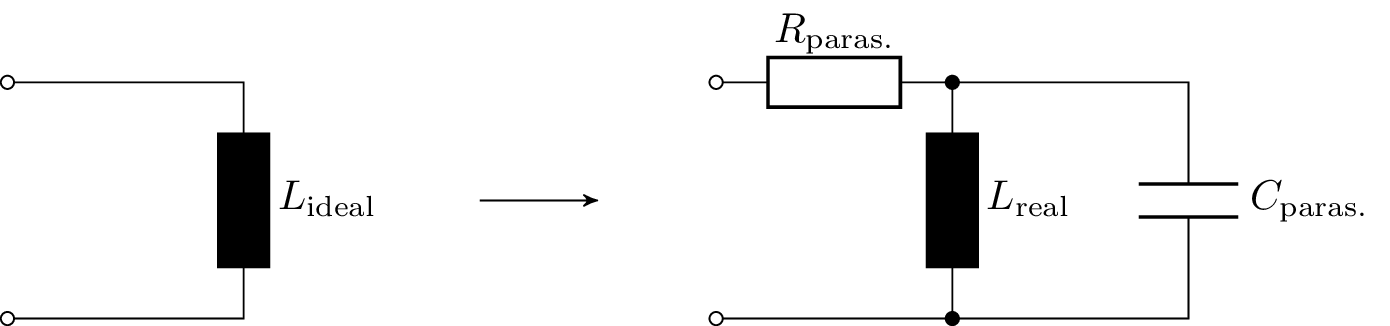
Like ohmic resistance and capacitors, real coils exhibit parasitic effects. The coil wire has an ohmic component (\(R_\mathrm {paras.}\)) that affects the complex impedance of the coil. In addition, the winding of the coil generates capacitive effects (\(C_\mathrm {paras.}\)). Figure 7 shows the equivalent circuit diagram of an ideal coil and a real coil.

5 Sources of alternating quantities

As with sources of direct current and direct voltage, there are alternating current sources with comparable characteristics. In an ideal alternating voltage source, the voltage is fixed. The alternating voltage does not change depending on the current flowing through it. The ideal alternating current source provides a fixed current . This is not influenced by the connected load. The circuit symbols for an ideal alternating voltage source and an ideal alternating current source are shown in Figure 8.

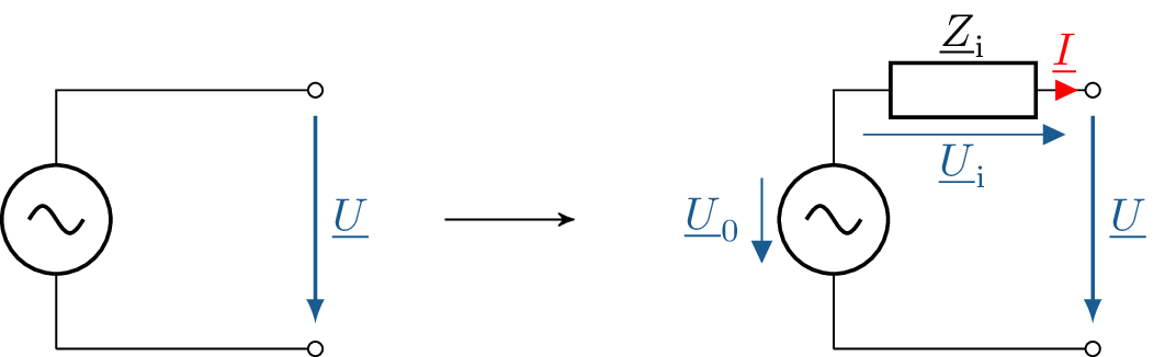
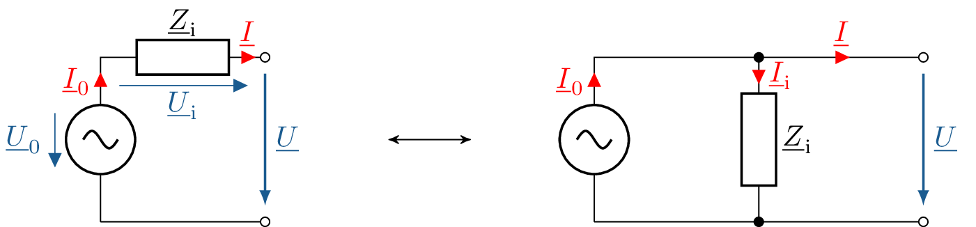
The two alternating current sources presented here are ideal sources. Real alternating current sources, like sources of direct voltage and direct current, have internal resistance. This internal resistance manifests itself in sources of alternating quantities as complex impedances. The real alternating voltage source therefore has a complex internal impedance \(\underline {Z}_\mathrm {i}\), which is connected in series with an ideal alternating voltage source. In real alternating voltage sources, the output voltage \(\underline {U}\) depends on the connected load. The comparison between an ideal and a real alternating voltage source is shown in Figure 9.

The output voltage of a real AC voltage source can be determined using equation 15. Here, the AC voltage of the AC voltage source is not directly applied to the terminals. It is reduced by the voltage across the internal impedance \(Z_\mathrm {i}\).

\begin {equation} \underline {U} = \underline {U}_\mathrm {0} - \underline {Z}_\mathrm {i} \cdot \underline {I} \label {GleichungQuel1} \end {equation}

Real AC voltage sources exhibit certain characteristics when unloaded, at no load and in the event of a short circuit. When idle, there is an infinite impedance between the terminals. No closed circuit is formed and no current flows (equation 16). The entire voltage of the AC source is applied to the open terminals, see equation 17.

\begin {equation} \underline {I} = 0 \qquad \rightarrow \qquad \underline {U}_\mathrm {i} = \underline {I} \cdot \underline {Z}_\mathrm {i} = 0 \label {GleichungQuel2} \end {equation} \begin {equation} \underline {U}_\mathrm {0} - \underline {U}_\mathrm {i} - \underline {U} = 0 \qquad \rightarrow \qquad \underline {U} = \underline {U}_\mathrm {0} \label {GleichungQuel3} \end {equation}

In the event of a short circuit, the impedance between the terminals approaches zero and there is no voltage drop. This results in the maximum possible short-circuit current, which is limited only by the internal impedance (equation 18). The voltage of the AC voltage source thus acts in its entirety across the internal impedance (Equation 19). The short-circuit current can be determined according to Equation 20 from the ratio of the voltage across the internal impedance \(\underline {U}_\mathrm {i}\) and the internal impedance \(\underline {Z}_\mathrm {i}\).

\begin {equation} \underline {U} = 0 \qquad \rightarrow \qquad \underline {I} = \underline {I}_\mathrm {k} \label {GleichungQuel4} \end {equation} \begin {equation} \underline {U}_\mathrm {0} - \underline {U}_\mathrm {i} - \underline {U} = 0 \qquad \rightarrow \qquad \underline {U}_\mathrm {i} = \underline {U}_\mathrm {0} \label {GleichungQuel5} \end {equation} \begin {equation} \underline {I}_\mathrm {k} = \frac {\underline {U}_\mathrm {i}}{\underline {Z}_\mathrm {i}} \label {GleichungQuel6} \end {equation}

Real Voltage sourceReal voltage source:

A real voltage source (230 V, 50 Hz) has an internal impedance \(\underline {Z}_\mathrm {i}\) as shown in the figure below, which consists of a coil \(L=20\ mH\) and an ohmic resistance \(R=10\ m\Omega \).

Determine the open-circuit voltage and the short-circuit current AC voltage source.

\begin {align} \underline {U}_\mathrm {0} &= 230\ V \cdot e^{\mathrm {j}0^o} \nonumber \\ \underline {Z}_\mathrm {i} &= R + j X_L \nonumber \\ \underline {Z}_\mathrm {i} &= 0,01\ \Omega + j \cdot 2\pi \cdot 50\ Hz \cdot 20\ mH \nonumber \\ \underline {Z}_\mathrm {i} &= 0,01\ \Omega + j 6,28\ \Omega \nonumber \end {align}

Open-circuit voltage: \begin {align} \underline {U} &= \underline {U}_\mathrm {0} \nonumber \\ \underline {U} &= 230\ V \cdot e^{\mathrm {j}0^o} \nonumber \end {align}

Short-circuit current: \begin {align} \underline {I}_\mathrm {k} &= \frac {\underline {U}_\mathrm {0}}{\underline {Z}_\mathrm {i}} \nonumber \\ \underline {I}_\mathrm {k} &= \frac {230\ V \cdot e^{\mathrm {j}0^o}}{0,01\ \Omega + j 6,28\ \Omega } \nonumber \\ \underline {I}_\mathrm {k} &= (0,058 - j36,6)\ A = 36,6\ A \cdot e^{-\mathrm {j}89,9^o} \nonumber \end {align}

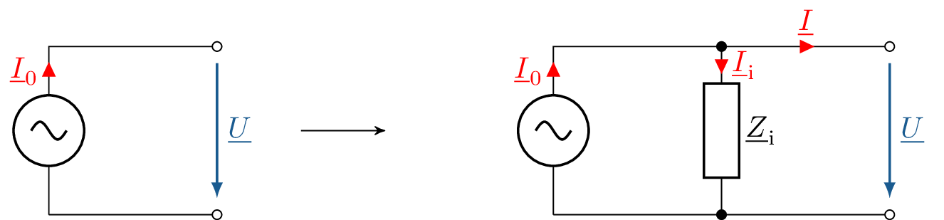
Like the AC voltage source, the real AC source in Figure 11 has an internal impedance \(\underline {Z}_\mathrm {i}\), whereby this internal impedance is not connected in series as in the AC voltage source, but rather in parallel to an ideal AC source. The resulting output current \(\underline {I}\) of the source depends on the connected load or the output voltage \(\underline {U}\).

The alternating current of the ideal alternating current source is reduced by a portion due to the internal impedance. The output current of the real alternating current source can be determined using equation 21. Here, starting from the source current \(\underline {I}_\mathrm {0}\), the output voltage-dependent (\(\underline {U}\)) alternating current component \(\underline {I}_\mathrm {i}\) is subtracted by the internal impedance \(\underline {Z}_\mathrm {i}\).

\begin {equation} \underline {I} = \underline {I}_\mathrm {0} - \underline {I}_\mathrm {i} = \underline {I}_\mathrm {0} - \frac {\underline {U}}{\underline {Z}_\mathrm {i}} \label {GleichungQuel7} \end {equation}

AC conversion

Alternating current and alternating voltage sources can be converted into each other if both alternating sources have the same short-circuit current and the same open-circuit voltage.

Both AC sources are equivalent if, according to Equation 22 and Equation 23, Ohm’s law applies with identical internal impedances for the AC voltage source and the AC current source.

\begin {equation} \underline {U}_\mathrm {0} = \underline {Z}_\mathrm {0} \cdot \underline {I}_\mathrm {0} \label {GleichungQuel8} \end {equation} \begin {equation} \underline {Z}_\mathrm {i} = \underline {Z}_\mathrm {0} \label {GleichungQuel9} \end {equation}

Here, the short-circuit current \(\underline {I}_\mathrm {K}\) should be equal to the source current \(\underline {I}_\mathrm {0}\) of the alternating current source, which is identical to the output current \(\underline {I}\). The output alternating voltage \(\underline {U}\) of the alternating sources corresponds to the open-circuit voltage \(\underline {U}_\mathrm {L}\).

\begin {equation} \underline {I} = \underline {I}_\mathrm {k} = \underline {I}_\mathrm {0} \qquad \text {und} \qquad \underline {U} = \underline {U}_\mathrm {L} = \underline {U}_\mathrm {0} \label {GleichungQuel10} \end {equation}

AC conversionAlternating current conversion:

Given is a real AC voltage source with \(\underline {U}_\mathrm {0} = 20\ kV \cdot \mathrm {e}^{\mathrm {j}30^o}\) and \(\underline {Z}_\mathrm {0} = (0.01 + j \cdot 2)\ \Omega \). Convert the alternating voltage source into an equivalent alternating current source and calculate the short-circuit current.

Short-circuit current:

\begin {equation} \underline {I}_\mathrm {0} = \frac {\underline {U}_\mathrm {0}}{\underline {Z}_\mathrm {0}} = \frac {20\ kV \cdot \mathrm {e}^{\mathrm {j}30^o}}{(0,01 + j \cdot 2)\ \Omega } = (5,04 + j \cdot 8,64)\ kA \nonumber \end {equation}

6 Complex voltage divider and complex current divider

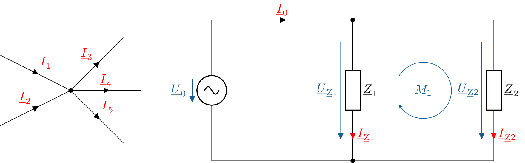
As with the consideration of direct current networks, the basic laws for analysing alternating current networks apply. The node rule and the mesh rule are to be applied equivalently here. The example node and the example mesh already presented are shown once again in Figure 13 with complex alternating quantities. This results in the formulation of the following equation 26 as an example of the complex node rule:

\begin {equation} \sum _{k = 1}^{N}{\underline {I}_\mathrm {k}} = 0 = \underline {I}_\mathrm {1} + \underline {I}_\mathrm {2} - \underline {I}_\mathrm {3} - \underline {I}_\mathrm {4} - \underline {I}_\mathrm {5} \label {KnotenregelKomplex} \end {equation}

As well as equation 27 as an example of the complex mesh rule:

\begin {equation} \sum _\mathrm {k = 1}^{N}{\underline {U}_\mathrm {k}} = \underline {U}_\mathrm {Z2} - \underline {U}_\mathrm {Z1} = 0 \label {MaschengleichungKomplex} \end {equation}

In contrast to direct current analysis, where only real values are used in calculations, here it is only necessary to ensure that complex alternating quantities are used.

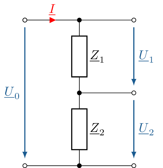
The complex voltage divider is used to reduce a total voltage, e.g. to adjust a signal level to the input voltage range of a measuring circuit. Figure 14 shows a complex voltage divider consisting of two complex impedances. The complex total voltage \(\underline {U}_\mathrm {0}\) is divided into the partial voltages \(\underline {U}_\mathrm {1}\) and \(\underline {U}_\mathrm {2}\) via the two impedances \(\underline {Z}_\mathrm {1}\) and \(\underline {Z}_\mathrm {2}\).

The total voltage is divided in proportion to the complex impedances (see Equation 28). Based on the complex current \(\underline {I}\) flowing through the entire series connection, the complex partial voltages \(\underline {U}_\mathrm {1}\) and \(\underline {U}_\mathrm {2}\) and their complex impedances \(\underline {Z}_\mathrm {1}\) and \(\underline {Z}_\mathrm {2}\) can be determined in relation to the complex total voltage \(\underline {U}_\mathrm {0}\) and the total complex impedance \(\underline {Z}_\mathrm {1} + \underline {Z}_\mathrm {2}\) can be determined.

\begin {equation} \underline {I} = \frac {\underline {U}_\mathrm {0}}{\underline {Z}_\mathrm {1} + \underline {Z}_\mathrm {2}} = \frac {\underline {U}_\mathrm {1}}{\underline {Z}_\mathrm {1}} = \frac {\underline {U}_\mathrm {2}}{\underline {Z}_\mathrm {2}} \label {GleichungTeiler1} \end {equation}

By rearranging equation 28, the complex partial ratio \(\underline {T}\) for equation 29 can be established:

\begin {equation} \underline {T} = \frac {\underline {U}_\mathrm {2}}{\underline {U}_\mathrm {0}} = \frac {\underline {Z}_\mathrm {2}}{\underline {Z}_\mathrm {1} + \underline {Z}_\mathrm {2}} \label {GleichungTeiler2} \end {equation}

Here, the ratio of the complex partial voltage \(\underline {U}_\mathrm {2}\) and the complex total voltage \(\underline {U}_\mathrm {0}\) corresponds to the ratio of the complex impedance \(\underline {Z}_\mathrm {2}\) and the total complex impedance of the series connection \(\underline {Z}_\mathrm {1} + \underline {Z}_\mathrm {2}\). The complex partial ratio can be established in the same way for the complex partial voltage \(\underline {U}_\mathrm {1}\).

The complex voltage divider is used, for example, in ohmic-capacitive dividers in high-voltage technology. Figure 15 shows four different dividers that are used, for example, in high-voltage technology.

In addition to the ohmic-capacitive divider, the ohmic divider, the capacitive divider and the damped capacitive divider are also presented. The ohmic divider consists purely of ohmic resistors, which are connected in series, and the capacitive divider consists purely of capacitors. The damped capacitive divider consists of several modules with an upstream coil. The modules are composed of series connections of an resistive resistor and a capacitor.

A simple example of such an ohmic-capacitive divider is shown in Figure 16. The ohmic-capacitive divider consists of at least two parallel circuits connected in series, each comprising an ohmic resistor and a capacitor, known as an RC element . In Figure 16, the first RC element consists of the resistor \(R_1\) and the capacitor \(C_1\). The second RC element consists of the resistor \(R_2\) and the capacitor \(C_2\). The complex total voltage \(\underline {U}_\mathrm {0}\) is applied across both RC elements. The complex partial voltage \(\underline {U}_\mathrm {2}\) is applied across the second RC element. The partial ratio therefore has ohmic and capacitive components. The capacitance of the capacitor results in a frequency-dependent partial ratio.

A special condition exists when the complex voltage divider is balanced. This condition describes the identical ratio of the components to each other. This condition is described by equation 30. Here the product of the resistor \(R_1\) and the capacitor \(C_1\) must be identical to the product of the resistor \(R_2\) and the capacitor \(C_2\). In practice, this balancing condition can be achieved using variable components such as trimmer capacitors.

\begin {equation} R_1 \cdot C_1 = R_2 \cdot C_2 \label {GleichungTeiler3} \end {equation}

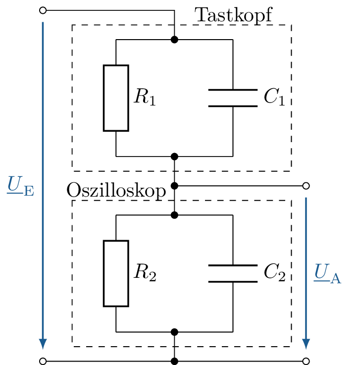
Another example of an ohmic-capacitive divider is the probe of an oscilloscope. Such a divider is shown in Figure 17. In principle, the image does not differ significantly from the ohmic-capacitive divider. However, here the first and second RC elements are spatially separated from each other and enclosed in a housing. The first RC element represents the probe and the second RC element represents the circuitry in the oscilloscope. With the ohmic division ratio:

\begin {equation} \frac {\underline {U}_\mathrm {A}}{\underline {U}_\mathrm {E}} = \frac {R_\mathrm {2}}{R_\mathrm {1}+R_\mathrm {2}} \end {equation}

and the capacitive ratio: \begin {equation} \frac {\underline {U}_\mathrm {A}}{\underline {U}_\mathrm {E}} = \frac {C_\mathrm {2}}{C_\mathrm {1}+C_\mathrm {2}} \end {equation}

To calibrate the probe, the ohmic and capacitive division ratios can be equated, as the division ratios must be identical: \begin {equation} \frac {R_\mathrm {2}}{R_\mathrm {1}+R_\mathrm {2}} = \frac {C_\mathrm {2}}{C_\mathrm {1}+C_\mathrm {2}} \end {equation}

The adjustment condition according to equation 30 still applies. The divider is adjusted via the adjustable capacitance \(C_1\).

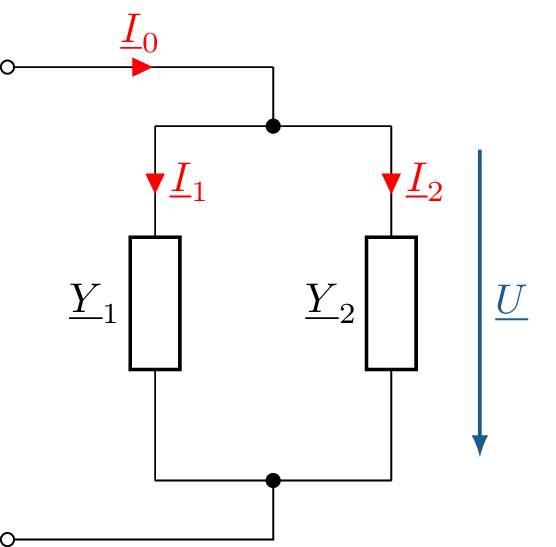
The complex current divider, as shown in Figure 18, divides the complex total current \(\underline {I}\) into the partial currents \(\underline {I}_\mathrm {1}\) and \(\underline {I}_\mathrm {2}\). The two partial currents \(\underline {I}_\mathrm {1}\) and \(\underline {I}_\mathrm {2}\) flow through the admittances \(\underline {Y}_\mathrm {1}\) and \(\underline {Y}_\mathrm {2}\).

The complex voltage \(\underline {U}\) can be calculated according to Equation 34 using the ratio of the total current \(\underline {I}\) and the total admittance \(\underline {Y}_\mathrm {1} + \underline {Y}_\mathrm {2}\) or using the ratios of the individual current branches:

\begin {equation} \underline {U} = \frac {\underline {I}_\mathrm {0}}{\underline {Y}_\mathrm {1}+\underline {Y}_\mathrm {2}} = \frac {\underline {I}_\mathrm {1}}{\underline {Y}_\mathrm {1}} = \frac {\underline {I}_\mathrm {2}}{\underline {Y}_\mathrm {2}} \label {GleichungStromteiler1} \end {equation}

The division ratio can be defined for the two current branches according to equation ??:

\begin {align} \underline {T}_\mathrm {i1} = \frac {\underline {I}_\mathrm {1}}{\underline {I}_\mathrm {0}} = \frac {\underline {Y}_\mathrm {1}}{\underline {Y}_\mathrm {1}+\underline {Y}_\mathrm {2}} \label {GleichungStromteiler2} \\ \underline {T}_\mathrm {i2} = \frac {\underline {I}_\mathrm {2}}{\underline {I}_\mathrm {0}} = \frac {\underline {Y}_\mathrm {2}}{\underline {Y}_\mathrm {1}+\underline {Y}_\mathrm {2}} \label {GleichungStromteiler3} \end {align}