Apparent power, active power and reactive power

In the direct current analysis of electrical networks, only active power was found at the components. In the alternating current analysis of electrical networks, the resulting reactive currents also generate reactive power. The resulting apparent power is divided between active power and reactive power. The following fundamentals and types of power caused by alternating voltage are discussed below:

1 Fundamentals: Addition theorem and arithmetic mean

An addition theorem has already been presented for calculating the RMS value. Another addition theorem is presented in equation 1. Here, the product of two sine functions with different arguments is related to sums and differences in cosine functions. This eliminates the product and creates a sum of two cosine functions. Integrating the sum can be simplified by dividing the sum into two separate integration processes.

\begin {equation} \sin (x) \cdot \sin (y) = \frac {1}{2} (\cos (x-y) + cos(x+y)) \label {GleichungAdd1} \end {equation}

The arithmetic mean of a function is used to calculate a constant value that is no longer time-dependent. In electrical engineering, this value is used in certain cases, similar to the RMS value for sinusoidal current and voltage curves, for better illustration. The arithmetic mean is calculated using the following integral formula:

\begin {equation} \overline {u(t)}=\frac {1}{T}\int _{t}^{t+T} u(t)dt \label {ArythMittel} \end {equation}

In the formula, \(T\) stands for the period length. Here, \(t\) is any freely selectable point in time from which the observation should start (usually \(t=0\)). Put simply, the integral represents the area between the function curve and the abscissa and the denominator of the fraction represents the period length. As an example, let us consider a so-called sawtooth voltage, which is shown in Figure 1.

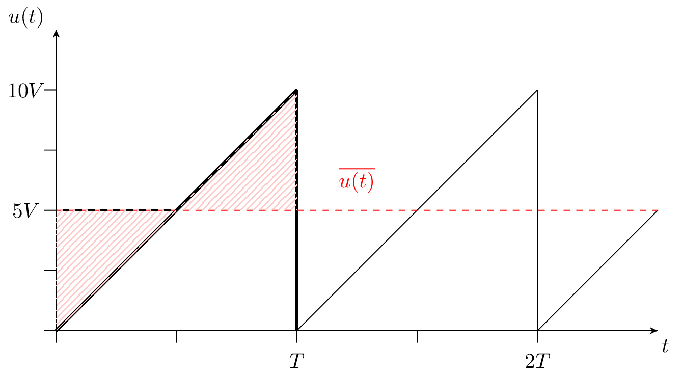
To calculate the arithmetic mean, a function must first be established over a period. In this case, a period can be expressed as follows:

\begin {equation} \overline {u(t)}=\frac {10~V}{T}\cdot t \end {equation}

Inserting this relationship into equation 2 and setting the integration limits \(t=0\) to \(T\) yields the equation:

\begin {equation} \overline {u(t)}=\frac {1}{T}\int _{0}^{T} \frac {10~V}{T}\cdot t~dt \end {equation}

When the integral is resolved, the arithmetic mean value for the sawtooth voltage is obtained:

\begin {equation} \overline {u(t)}=\frac {1}{T}\left [\frac {10~V}{T}\cdot \frac {t^2}{2}\right ]_0^T=\frac {1}{2}\cdot 10~V \end {equation}

The arithmetic mean is therefore half the maximum voltage. In the case of an ideal sine wave, the arithmetic mean is always zero. The arithmetic mean is relevant when the power of sinusoidal currents and voltages is to be calculated.

2 Active power and reactive power

Active power in direct current: In direct current electrical networks, power is determined using the well-known equation \(P=U\cdot I\). If the electrical resistance is known, the equation can be rearranged so that, according to Ohm’s law, either the voltage or the current is eliminated. Active power in alternating current:

\begin {equation} P = U \cdot I = I^2 \cdot R = \frac {U^2}{R} \label {GleichungLei1} \end {equation}

In a system with alternating quantities, power, like current and voltage, is time-dependent. In equation 7, this is expressed by the fact that the symbols are written in lower case and are dependent on time \(t\):

\begin {equation} P = U \cdot I \Leftrightarrow p(t)=u(t)\cdot i(t) \label {GleichungLei2} \end {equation}

Because the magnitude of voltage and current are time-dependent, this function of power is also time-dependent. Due to its time dependency, we also refer to Augenblicksleistung for a given point in time t. The unit of measurement for instantaneous electrical power continues to be the watt.

\begin {equation} u(t)=\hat {U}\cdot \sin (\omega t + \varphi _\mathrm {U}) \qquad i(t)=\hat {I}\cdot \sin (\omega t + \varphi _\mathrm {I}) \label {GleichungLei3} \end {equation}

If the instantaneous values of voltage and current are substituted into equation 7 for instantaneous power, the following equation ?? gives the instantaneous power. Here, the equation can be divided into a leading factor, a constant component and a time-dependent component. The pre-factor consists of half the product of the amplitude values of voltage and current. The constant part consists of the first cosine summand; here, only the phase angles of voltage and current are decisive. The time-dependent part is represented by the second cosine. Here, in addition to the phase angles, the angular frequency and the time are also important.

\begin {align} \text {Generally:} p(t) &= u(t) \cdot i(t) \\ \text {Sinusoidal:} p(t) &= \frac {\hat {U}\cdot \hat {I}}{2}(\underbrace {\cos (\varphi _\mathrm {U}-\varphi _\mathrm {I})}_\text {constant proportion} + \underbrace {\cos (2\omega t +\varphi _\mathrm {U}+\varphi _\mathrm {I})}_\text {time-dependent portion}) \label {GleichungLei4} \end {align}

If the entire power of a system is absorbed via an ideal ohmic resistor, this means that the voltage in the current has no phase shift. The constant component of the instantaneous power is positive. The instantaneous power pulsates at twice the frequency compared to the frequency of the voltage and current. In this case, the power always has a positive sign.

Often, the exact temporal course of the instantaneous power is not significant. Rather, in applications only the average power converted, for example heat applications, is of interest. The average power of the time-varying instantaneous power is defined by equation 2. For purely sinusoidal voltages and currents, the average power can be determined using equation 10. The voltage \(U\) and current \(I\) values are the RMS value. The angle \(\varphi \) results from the phase shift between the voltage and the current. The entire expression \(\bf \cos (\varphi )\) is also referred to as the Leistungsfaktor.

\begin {equation} \overline {p}_\mathrm {Sin} = P = U \cdot I \cdot \cos (\varphi ) \label {GleichungLei5} \end {equation}

Without the phase shift between the voltage and the current at an ideal resistor, the power factor term is negligible. Thus, in alternating current technology, the average power can be reduced to two time-independent variables in the case of sinusoidal voltage and current curves, analogous to direct current technology. The RMS value of the voltage and current are used to determine the average power for purely sinusoidal quantities.

\begin {equation} \overline {p}_\mathrm {Ohm} = \frac {\hat {U}}{\sqrt {2}} \cdot \frac {\hat {I}}{\sqrt {2}} = \frac {\hat {U}\cdot \hat {I}}{2} = U \cdot I \label {GleichungLei6} \end {equation}

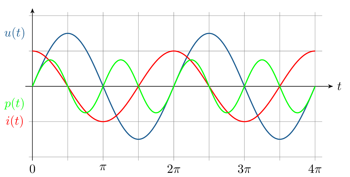
The situation is similar with the instantaneous power at coils and capacitors. At an inductance, the current lags the voltage by 90° (\(+\pi /2\)). The voltage and current waveforms across an inductance are shown in Figure 2. The instantaneous power across the inductance is shown in green. The constant component of the instantaneous power across an inductance is zero. The curve shows the pulsation of the instantaneous voltage with twice the frequency of the voltage or current. The positive and negative half-waves of the instantaneous power cancel each other out on average. This means that the power consumed is completely re-emitted and thus no power is consumed by the inductance.

In principle, the capacitor behaves in the same way as inductance. Here, the current lags the voltage by 90° (\(-\pi /2\)). The constant component of the instantaneous power is zero and the power pulsates at twice the frequency around the zero line. As with inductance, the power absorbed by a capacitor is completely re-emitted, so that on average no power is absorbed. The behaviour of time-dependent power at a capacitive load is shown in Figure 3.

If the instantaneous power is greater than zero, power is absorbed. Conversely, power is delivered when the instantaneous power is less than zero. Due to the absence of phase shift between the current and voltage at the ohmic resistor, the average power is always greater than zero. The ohmic resistance therefore always consumes power. The power is referred to here as active power \(P\), which can be used for applications. It is calculated using the equation 10 already presented for sinusoidal voltages and currents. The powers described explain active power components and reactive power components. Reactive power describes the portion of power that is necessary for the generation of electric and magnetic fields. If the electrical impedance is purely inductive or capacitive, there is a phase shift of \(\pm 90^\circ \). The purely inductive or purely capacitive two-pole absorbs power, which is then completely released again. The resulting mean power is always zero. This power is referred to as reactive power \(Q\). A distinction is made between inductive and capacitive reactive power. For inductive reactive power, there is a positive phase shift for the power, which corresponds exactly to the course of the sine function. The capacitive reactive power is shifted in the opposite direction, so that a sine function can also be defined, but with a negative sign. Equations 12 and 13 present the equations for calculating inductive and capacitive reactive power. The unit of measurement for inductive and capacitive reactive power is the var (volt-ampere reactive).

\begin {equation} Q_\mathrm {Ind} = U \cdot I \cos (\varphi + 90^\circ ) = U \cdot I \cdot \sin (\varphi ) \label {GleichungLei7} \end {equation}

\begin {equation} Q_\mathrm {Kap} = U \cdot I \cos (\varphi - 90^\circ ) = - U \cdot I \cdot \sin (\varphi ) \label {GleichungLei8} \end {equation}

\begin {equation} [Q] = 1\ Volt-Ampere-reactive = 1\ \mathrm {var} \nonumber \end {equation}

With ideal capacitive or inductive resistors, no energy is converted into heat. Only the magnetic or electric field changes, so energy is stored or released.

3 Apparent power

So far, we have looked at the basics of power analysis for ideal ohmic and inductive/capacitive impedances. However, most networks contain both ohmic and inductive or capacitive impedances. In such networks, a distinction is made between apparent power, active power and reactive power. The apparent power represents the total power of the system. To calculate the apparent power, the maximum value is used, i.e. when there is no phase shift. This value is therefore equal to the power of an ideal ohmic resistor:

\begin {equation} S=U\cdot I = P_\mathrm {R} \label {s} \end {equation}

If the apparent power is considered in the complex plane, the fixed pointers are used. If the complex voltage is multiplied by the complex current, the phase angles would be added according to the rules of complex arithmetic. However, in order to perform a correct power calculation, there must be a difference between the phase angles. To remedy this problem, the conjugate complex value of the current is used in the calculation:

\begin {align} \underline {S}&=\underline {U}\cdot \underline {I}^* \nonumber \\ with~~~ \underline {U}&=U\cdot e^{j\varphi _\mathrm {u}} \nonumber \\ and~~~ \underline {I}^*&=I\cdot e^{-j\varphi _\mathrm {i}} \\ follows~~~ \underline {S}&=U\cdot e^{j\varphi _\mathrm {u}} \cdot I\cdot e^{-j\varphi _\mathrm {i}}\nonumber \\ &=U\cdot I\cdot e^{j(\varphi _\mathrm {u}-\varphi _\mathrm {i})} \\ &=U\cdot I\cdot e^{j(\varphi )} \nonumber \end {align}

The complex value of the voltage and the conjugate complex value of the current can be used to determine the active power and the reactive power separately, or the complex apparent power directly:

\begin {equation} U \cdot I \cdot e^{j\varphi }=U\cdot I\cdot (\cos \varphi +j~\sin \varphi )=P+jQ=\underline {S} \end {equation}

In addition, the power factor can also be used to directly determine a relationship between the active power or reactive power and the apparent power according to Equation 18.

\begin {equation} P = \cos (\varphi ) \cdot S \qquad \qquad Q=S\cdot \sin (\varphi ) \label {GleichungSch1} \end {equation}

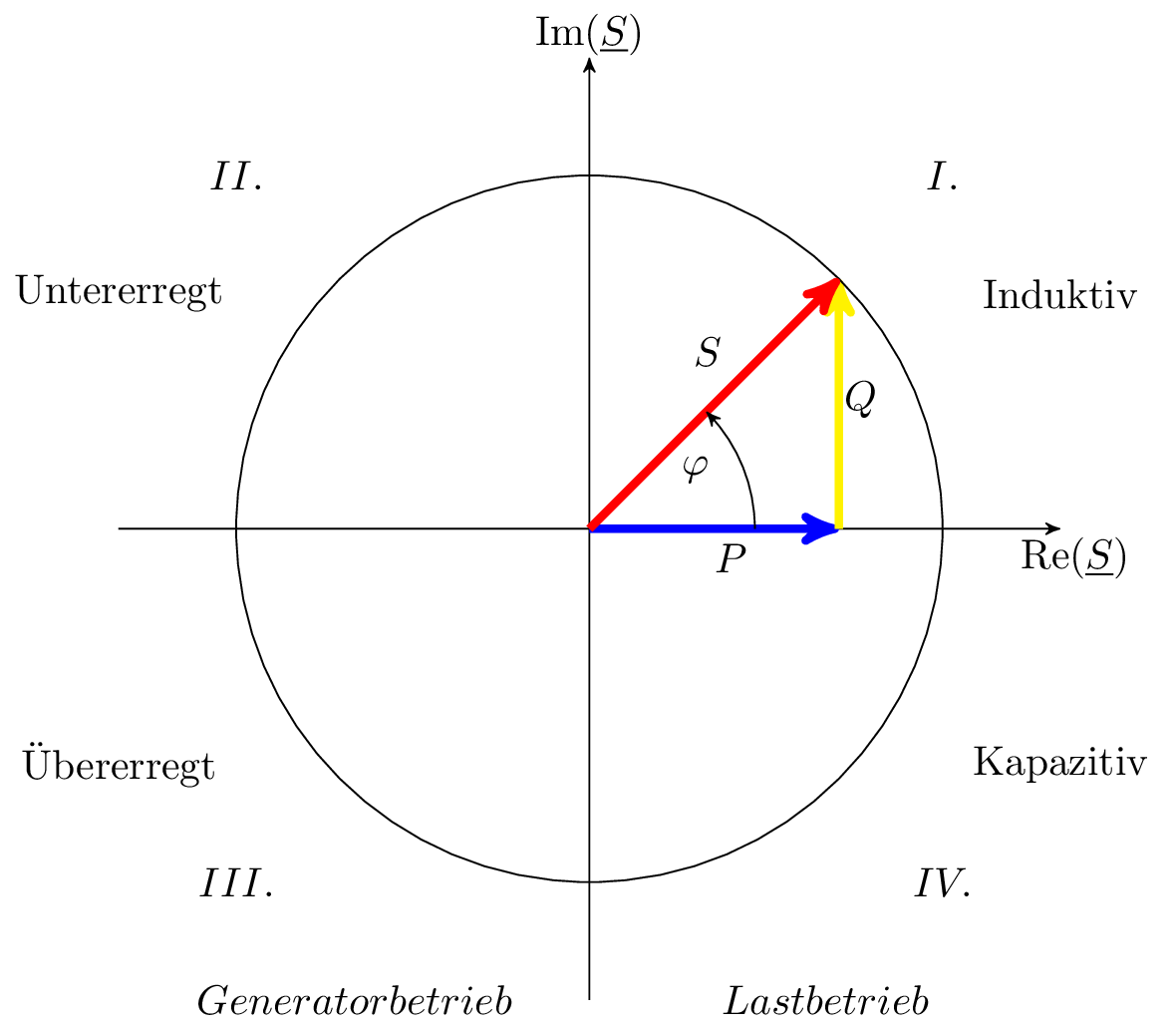
The quantities active power and reactive power are found in the complex number plane. Active power is a purely real value, while reactive power is a purely imaginary value. Apparent power, which is also a complex quantity, can be represented as the sum of active and reactive power (see Figure 4). The apparent power \(S\) shown here with the associated phase angle \(\varphi \) is located in the \(I\) quadrant. This is caused by a positive active power component and a positive reactive power component. The positive active power indicates that some electrical power is being consumed, i.e. it represents an electrical load. This is why we refer to load operation here. The positive reactive power indicates the prevailing effects of a coil and thus has an inductive effect. The apparent power in the first quadrant is operated in inductive load mode. If a negative active power affects the apparent power, active power is delivered, as in the case of a generator that delivers power. With positive reactive power, inductive generator operation occurs (quadrant II). If the reactive power is negative, capacitive effects predominate. With negative active power, this type of operation is called capacitive generator operation (quadrant III). Finally, capacitive load operation is described in the \(IV.\) quadrant. Here, positive active power and negative reactive power affect the apparent power.

Reactive power is needed, among other things, to generate magnetic fields in electrical machines. The reactive power requirement arises from components in the system that have either an inductive or capacitive effect. If the current required to generate the magnetic field (excitation current) is higher than would be necessary for the nominal power of the generator, the generator is overexcited. In this case, the generator is able to supply reactive power to the grid. The resulting increase in reactive power in the grid leads to a rise in voltage. If the energy demand in the grid increases, this situation can be used to counteract a drop in grid voltage. Conversely, a generator with a lower excitation current than required operates in an underexcited state. The generator draws reactive power from the grid in order to maintain the required magnetic field. The consumption of reactive power then leads to a voltage drop in the grid. Severe underexcitation of a generator can cause the electrical machine to fail.

The units of the three types of power are theoretically all comparable. In order to distinguish between the types of power, new units were chosen for apparent power and reactive power, which physically express the same thing. The unit volt-ampere [VA] was defined for apparent power and volt-ampere reactive [var] for reactive power. Active power is specified in the familiar unit of watts [W].

4 Power and electrical energy

In addition to electrical power, electrical energy is also a quantity used, for example, to record consumption in households. Here, the electrical power per unit of time is measured. According to the definition from thermodynamics, energy is the power applied over a certain period of time. So, according to equation 20, the electrical power during a time between \(t_1\) and \(t_2\) is integrated to determine the electrical energy.

\begin {equation} E_\mathrm {el} = \int _{t_1}^{t_2} p_\mathrm {el}(t)\ \mathrm {d}t \label {GleichungEne1} \end {equation}

Similar to active power and reactive power, energy can also be divided into active work and reactive work. Reactive work describes the portion of electrical energy that is not converted into useful energy or active work.

\begin {equation} W_\mathrm {N} = \int _{t_1}^{t_2} p(t) \ \mathrm {d}t \qquad \qquad W_\mathrm {Q} = \int _{t_1}^{t_2} Q \ \mathrm {d}t \label {GleichungEne2} \end {equation}

In a steady state, only the RMS value of voltage and current, and thus also of apparent power, active power and reactive power, are considered and are therefore constant over time.

\begin {equation} W_\mathrm {N} = P \cdot (t_2 - t_1) \qquad \qquad W_\mathrm {Q} = Q \cdot (t_2 - t_1) \label {GleichungEne3} \end {equation}

Power calculationPower calculation:

The following values for the alternating voltage and alternating current are measured on an alternating current load:

Given is: \begin {equation} \hat {U} = 12\ V \qquad \hat {I} = 2A\ \nonumber \qquad \varphi = 60^\circ \ \nonumber \end {equation}

The following tasks are to be completed:

• Calculation of active power and reactive power.
• Calculation of apparent power using the conjugate complex current.

a)

The active power is: \begin {align} P &= U \cdot I \cdot \cos (\varphi ) = \frac {\hat {U}}{\sqrt {2}} \cdot \frac {\hat {I}}{\sqrt {2}} \cdot \cos (\varphi ) = \frac {12\ V}{\sqrt {2}} \cdot \frac {2\ A}{\sqrt {2}} \cdot \cos (60^o) \nonumber \\ P &= 6\ W \nonumber \end {align} The reactive power is: \begin {align} Q &= U \cdot I \cdot \sin (\varphi ) = \frac {\hat {U}}{\sqrt {2}} \cdot \frac {\hat {I}}{\sqrt {2}} \cdot \sin (\varphi ) = \frac {12\ V}{\sqrt {2}} \cdot \frac {2\ A}{\sqrt {2}} \cdot \sin (60^o) \nonumber \\ Q &= 10,392\ var \nonumber \end {align}

b)

The apparent power is: \begin {align} \underline {S} &= \underline {U} \cdot \underline {I}^* = \frac {\underline {\hat {U}}}{\sqrt {2}} \cdot \frac {\underline {\hat {I}}^*}{\sqrt {2}} = \frac {12\ V}{\sqrt {2}} \cdot e^{j(2\pi \cdot 20\ Hz)} \cdot \frac {2\ A}{\sqrt {2}} \cdot e^{j(2\pi \cdot 20\ Hz+\frac {\pi }{3})} \nonumber \\ \underline {S} &= 12\ VA \cdot e^{j\frac {\pi }{3}} = 6\ W + j10,392\ var \nonumber \end {align}