

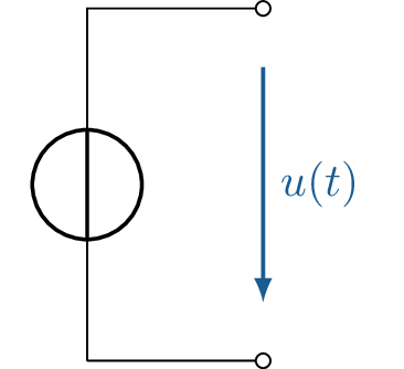
Voltage and current source
The operation of electrical devices is usually associated with the conversion of electrical power. In Module 2 on the topic of energy and power, we already learned that power corresponds to the amount of work done per unit of time and that this is equivalent to energy conversion. In order to operate electrical devices, in which energy is always converted, energy must be supplied. Energy can only be converted, not generated. Nevertheless, in electrical engineering, the supply of energy to the circuits under consideration is described with the aid of current and voltage sources. This does not take into account the fact that this involves the conversion of, for example, mechanical or chemical energy into electrical energy. However, this is irrelevant for the consideration of the circuit. The following section describes current and voltage sources and explains the differences between them.
Learning objectives: Voltage and current source
The Students can
- distinguish between voltage and current sources and know their circuit symbols.
- model real voltage and current sources.
- name examples of different sources.
1 Voltage sources
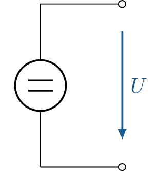
The most common type of energy source for electrical systems is the voltage source. Ideally, it is characterised by the fact that it outputs a constant voltage regardless of the connected load. Figure 1 shows the circuit symbol of an ideal voltage source with a constant output voltage \(U_{\mathrm {q}}\).
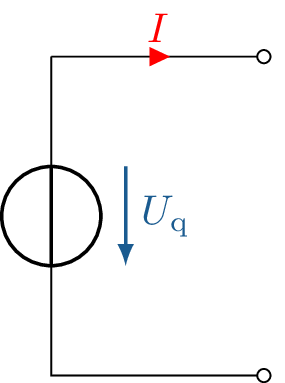
In Figure 1, the lines lead to nothing, which is referred to as open terminals. Since the circuit is not closed, no current flows. If the terminals were short-circuited in this case, the source would attempt to maintain the voltage and an infinitely high current would flow. Why this is so dangerous is explained in section 2 using a real voltage source as an example.
2 Modelling real voltage sources
Ideal components are always used in circuit diagrams, i.e. the graphical representation of electrical circuits. In order to be able to model the real behaviour of components correctly and thus replicate the real circuit behaviour as accurately as possible, the actual behaviour of the component must be replicated with the aid of ideal components. The following describes how the behaviour of a real voltage source can be replicated using ideal components. The technical implementation of any voltage source consists of physical components, all of which have specific resistance values. All these properties together result in the so-called internal resistance \(R_\mathrm {i}\) of a source. In the case of a real voltage source, the internal resistance is in series with the ideal voltage source. Figure 2 shows a modelled real voltage source.
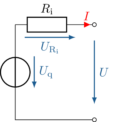
The circuit diagram shows that both \(U_\mathrm {q}\) and \(U\) point downwards. This is due to the counting arrow system, which is discussed in more detail in Module 4. At this point, it is sufficient to know that the generator counting arrow and the consumer counting arrow are opposite, since the sum of both arrows must be zero. If a consumer is now connected, the current flows through the internal resistance \(R_\mathrm {i}\) through the consumer. This means that power is also converted in the internal resistance.
If we consider the behaviour of short-circuited output terminals in a real-world scenario, the entire power delivered by the source is converted solely by the internal resistance of the voltage source. The power can be calculated using \(P = \frac {U^2}{R_{\mathrm {i}}}\). As a rule, the source is not designed for this, which would result in the energy being converted into a great deal of heat energy and lead to the destruction of the source.
If a load with a resistance \(R_{\mathrm {L}}\) is connected to the output of the voltage source, a current \(I\) flows through the resistors \(R_{\mathrm {i}}\) and \(R_{\mathrm {L}}\). This can be calculated according to Ohm’s law and the summary of resistors presented in the following module as \(I = \frac {U_{\mathrm {q}}}{(R_{\mathrm {i}} + R_{\mathrm {L}})}\). This current causes a voltage \(U_{\mathrm {R_{\mathrm {i}}}}\) to drop across the internal resistance \(R_{\mathrm {i}}\). In Module 2, it was already derived that the sum of all voltages within a closed circuit must be zero. In Module 4, the so-called mesh rule is derived from this, which can be used to calculate the output voltage \(U\) as
\begin {equation} U = U_{\mathrm {q}} - U_{\mathrm {R_{\mathrm {i}}}} = U_{\mathrm {q}} - I \cdot R_{\mathrm {i}} = U_{\mathrm {q}} - U_{\mathrm {q}} \cdot \frac {R_{\mathrm {i}}}{R_{\mathrm {i}} + R_{\mathrm {L}}} \end {equation}
The smaller the internal resistance \(R_{\mathrm {i}}\), the less the output voltage \(U\) of a loaded voltage source differs from the source voltage \(U_\mathrm {q}\). An internal resistance \(R_{\mathrm {i}}\) that is as small as possible in comparison to the load resistance \(R_{\mathrm {L}}\) should therefore be aimed for in order to achieve the most ideal behaviour possible. This can be achieved, among other things, by using the largest possible conductor cross-sections within the source.
If the real voltage source, modelled with \(U_\mathrm {q}\) and \(R_{\mathrm {i}}\), is operated in idle mode, the output voltage \(U\) is equal to the source voltage \(U_\mathrm {q}\), since no current flows through the internal resistance and no voltage can drop there.
Examples of real voltage sources include batteries and accumulators. As described above, the aim is to achieve the lowest possible internal resistance. A 12 V starter battery for cars has an internal resistance of less than 10 m\(\Omega \). A domestic power socket can also be regarded as a voltage source with a source voltage of 230 V and low internal resistance.
Key point:
- A voltage source must never be short-circuited!
- With voltage sources, the current always adjusts itself.
3 Current sources
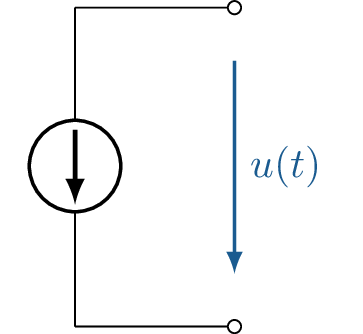
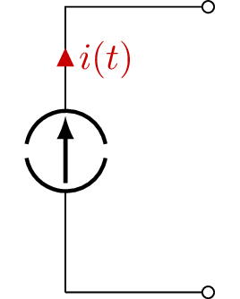
Compared to voltage sources, current sources are much less common. They are characterised by the fact that they supply a constant current and the voltage adjusts accordingly. Figure 3 shows the circuit symbol of an ideal current source with a constant output current. \(I_{\mathrm {q}}\).
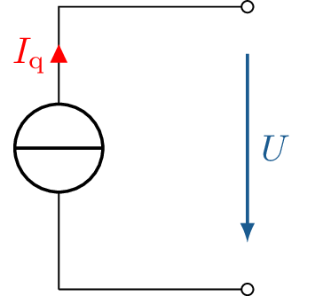
The case of an idle current source shown here leads, similarly to the short-circuited voltage source, to an infinitely high power output from the source and must therefore be avoided.
4 Modelling real current sources
Just as with voltage sources, there are no ideal current sources in reality. In order to describe the real behaviour of a current source, it must first be modelled. Figure 4 shows such a modelled current source.
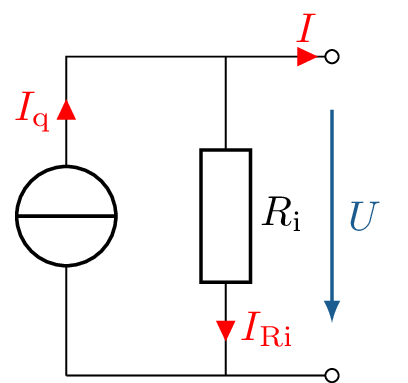
The model of the real current source also consists of the internal resistance \(R_\mathrm {i}\) and the ideal current source, where the difference to the voltage source is that the internal resistance is placed in parallel to the ideal current source. Here, too, the actual output current is smaller than the source current \(I_{\mathrm {q}}\). Module 4 introduces the node rule. This states that the sum of all currents in a node (branch point) must be zero, so that the output current \(I\) is given by
\begin {equation} I = I_{\mathrm {q}} - I_{\mathrm {R_{\mathrm {i}}}} = I_{\mathrm {q}} - \frac {U}{R_{\mathrm {i}}} \end {equation}
The greater the internal resistance \(R_{\mathrm {i}}\), the smaller the current \(I_{\mathrm {R_{\mathrm {i}}}}\) and the smaller the difference between the output current \(I\) and the source current \(I_{\mathrm {q}}\).
Contrary to the circuit diagram shown, a current source must never be operated with open terminals, as, similar to the case of a voltage source, the entire power would be converted in the internal resistance, which would lead to high thermal stress and ultimately to the destruction of the current source. Examples of real current sources are solar cells in the corresponding operating state or a laboratory power supply in current limiting mode.
Key point:
- A power source must never be operated in idle mode!
- With power sources, the voltage always adjusts itself.
5 Conversion of voltage and current sources
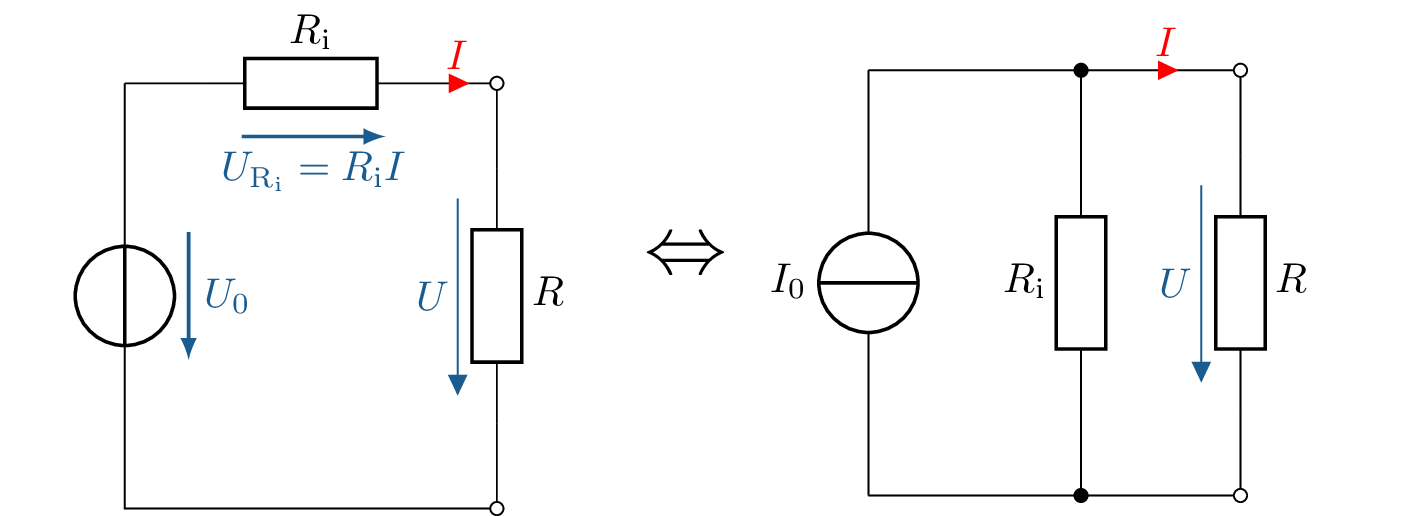
Voltage and current sources can be converted into each other with regard to their terminal behaviour. The prerequisite for this is that both the short-circuit current \(I_\mathrm {K}\) and the open-circuit voltage \(U_\mathrm {L}\) are the same for both sources. Figure 5 shows the conversion of the circuit diagrams into each other. Further information on conversion and power matching will follow in Module 4.
6 Various voltage and current sources
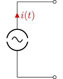
The previously introduced circuit symbols for voltage and current sources are universal and do not make any specific statements about the signal form of the output variable. In addition to the distinction between voltage and current sources, a fundamental distinction is also made between direct current (DC) and alternating current (AC).
The most common form for operating electronic devices is the direct voltage source. It continuously ensures that charge carriers flow from the negative to the positive pole, which generates a constant electric field from the positive to the negative pole.
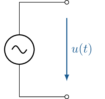
Alternating current (AC) sources, on the other hand, typically have a sinusoidal output voltage or a sinusoidal output current. In the past, high-voltage lines with alternating current have become the standard for transporting energy over long distances, as they were technically simpler and more cost-effective to implement. The most significant advantage of alternating current is the simple transformation of the voltage. It is also practical because there is no need to pay attention to polarity when connecting consumers.
However, the first implementations of energy transport in the form of direct current voltage are now
also available. The use of direct current (DC) for long transmission distances, such as in the
HVDC (High Voltage Direct Current) lines from the North Sea to southern Germany, offers a
number of advantages: Direct current is more efficient because it does not generate reactive
power, which means that there are no additional losses due to cable capacity. This keeps the
current amplitude lower, resulting in lower transmission losses and making DC particularly
attractive for very long distances. Figure 6 shows the circuit symbols for the various sources.
Voltage source
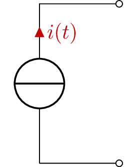
Current source
It should be noted that AC voltage and current sources have a sinusoidal output voltage or sinusoidal output current, whereas sources that can be varied arbitrarily over time can have any shape. One example of this is the square wave signal, which could originate from switching a DC voltage source on and off. Such sources are used, for example, in mobile applications of the widely used type of electric motors, which are also called synchronous or asynchronous machines. These motors are operated in mobile applications by a DC voltage source, whose signal shape is converted (pulsed) into the desired square wave signal with the aid of power electronics and a sinusoidal current is generated in the motor from the pulsed voltage signal via the coil windings. More on this in the module on electric machines. Another example of signals that can occur at any time is digital information transmission in communications engineering, where a one corresponds to a high signal and a zero to a low signal, which also resembles a square wave signal.
