

Capacity and capacitor
In electrical engineering, there are three basic components that can be used to describe the electrical behaviour of components. In addition to the ohmic resistance discussed above, there are also capacitance and inductance. This section deals with the property of capacitance and the associated component, the capacitor. The following section deals with inductance and the associated component, the coil.
Learning objectives: Capacity and capacitor
The Students
- can differentiate between capacity and capacitor.
- are familiar with the most important parameters relating to capacitors and capacitance.
- can calculate the capacity of a capacitor.
1 Electrical capacity \(C\)
Electrical capacity is the ability of an object to store electrical energy in the form of an electric field. This property occurs when electrical charge carriers are unevenly distributed and an electric field forms between the areas. The symbol for capacity is \(C\) (capacity), while the unit is given in farads (\(F\)).
The simplest and most common example used to explain capacitance is the plate capacitor. In this type of capacitor, two conductive plates are positioned opposite each other, each of which is charged with a different potential. Figure 1 shows a capacitor with an idealised field distribution.
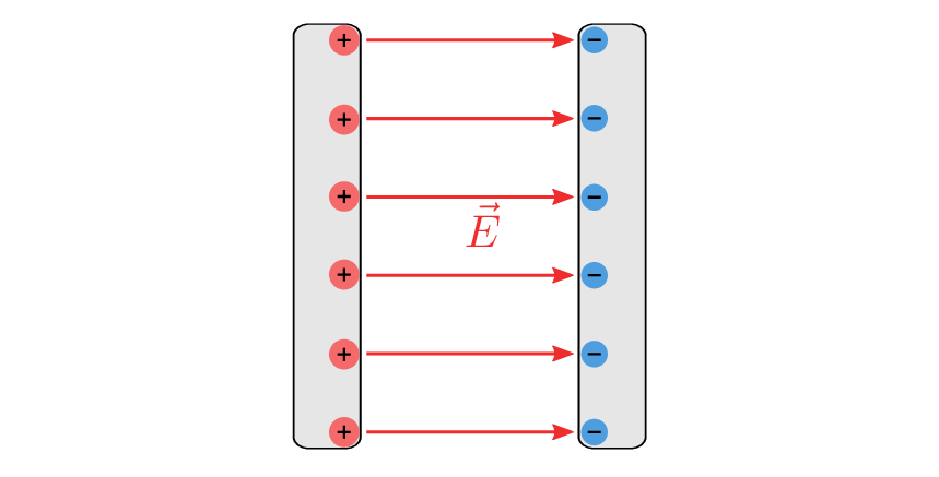
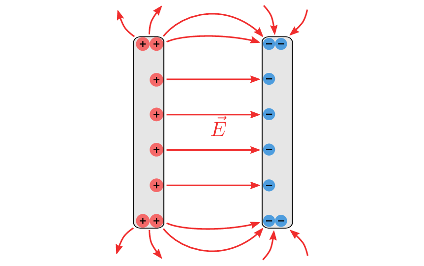
Due to the different potentials on the plates, an electric field forms from the higher to the lower charged plate. Ideally, it is assumed that no field forms outside the capacitor plates. In reality, charge carriers also accumulate at the side edges of the plates, leading to more complex field distributions. Figure 2 shows a diagram of such a real plate capacitor.
In many cases, however, the real behaviour can be neglected, which greatly simplifies the calculations. For this reason, only idealised capacitors will be considered in the following.
Capacitance is defined as the ratio of the stored electrical charge \(Q\) to the applied voltage \(U\). The higher the capacitance of a capacitor, the more charge it can store at a given voltage.
\begin {equation*} [C] = 1\, \text {Farad} = 1\, \text {F} = 1\,\, \frac {\text {C}}{\text {V}} = 1\, \frac {\text {A} \text {s}}{\text {V}} \label {eq:cqu} \end {equation*} \begin {equation} C = \frac {Q}{U} \end {equation} \begin {equation} Q = C \cdot U \Rightarrow C = \frac {Q}{U} = \frac {\varepsilon \cdot \iint \vec {E} \cdot \mathrm {d}\vec {A}}{\int \vec {E}\mathrm {d}\vec {s}} \label {eq:qcu2} \end {equation}
2 The capacitor as a component
The properties of capacitance are deliberately exploited in various areas of electrical engineering. These properties are utilised with the aid of capacitors. They are available in various designs. Figure 3 shows some examples, ranging from THT to SMD components.
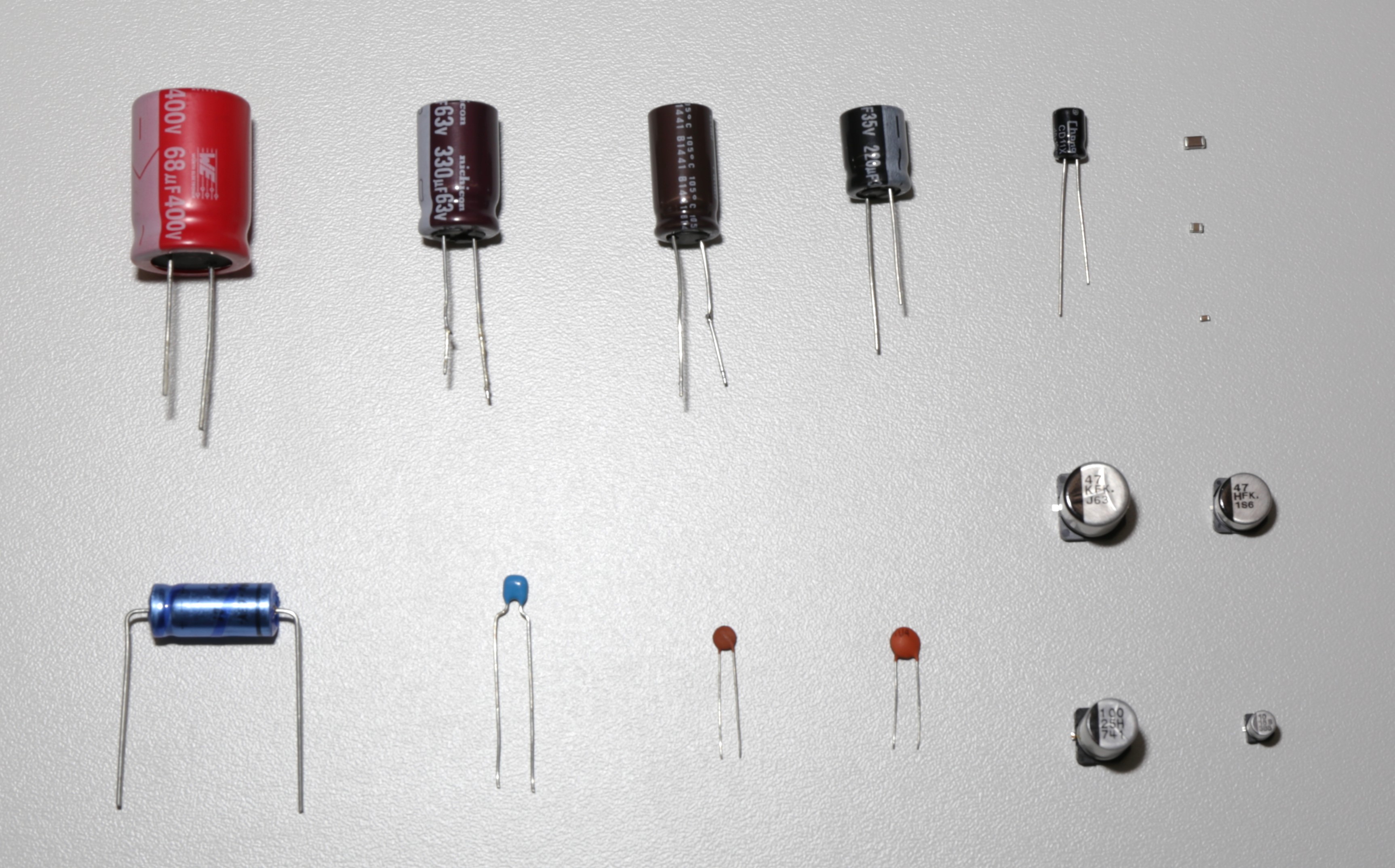
However, they are also available in significantly smaller or larger dimensions. In high-frequency technology, for example, capacitance is achieved solely through the design of the printed circuit boards, whilst capacitors for industrial or energy technology applications can be several centimetres to metres in size.
What all capacitors have in common is their ability to utilise the property of capacitance, as shown in the following circuit diagram 4. However, this circuit diagram only represents the idealised, usable capacitance.

For a realistic simulation of the circuit, it is important to describe the capacitor as a component in its entirety. This is done with the aid of an equivalent circuit diagram, which also simulates the unwanted, i.e. parasitic, properties of the component. Figure 5 shows such an equivalent circuit diagram.

The equivalent circuit diagram of the capacitor takes into account not only the usable capacitance, but also the parasitic properties that occur in real capacitors. These parasitic properties arise, for example, from the inductance of the connections and the ohmic losses in the material. The modelled equivalent circuit allows these effects to be taken into account in the circuit design and the switching behaviour to be better predicted.
Key point:
The capacitor is a desperate attempt to replicate a capacitance.
3 The dielectric
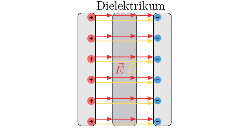
As the name implies, a dielectric is a dielectric material, i.e. one that does not conduct electricity. Since every material consists of atoms and all atomic nuclei are surrounded by electrons (electron shell), even a material that does not conduct electricity has an effect on the behaviour of the electric field. As soon as such a material is inserted between the plates of a capacitor, the properties of the capacitor also change. In Figure 6, the interrupted arrow of the electric field shows the different behaviour. The electric flux density D is an auxiliary quantity that is independent of the material and will be discussed in section 1.3.4.
The properties of the dielectric are material-specific and are quantified by the dielectric constant \(\varepsilon _\mathrm {r}\). Table 1 lists examples of some dielectrics and their \(\varepsilon _\mathrm {r}\):
| Material | \(\varepsilon _\mathrm {r}\) |
| Vacuum | 1 |
| Air (at STP) | 1.0006 |
| Plastic (PE) | 2.25-2.3 |
| Glass | 3-10 |
| Ceramics | 5-300 |
| Silicon | 11.7 |
| Tantalum oxide | 25-30 |
| Water | 81 |
In order to fully describe the material properties of the dielectric, the electric field constant \(\varepsilon _\mathrm {0}\) is required in addition to the dielectric constant. This refers to the dielectric behaviour of the electric field in a vacuum. While the dielectric constant \(\varepsilon _\mathrm {r}\) is dimensionless, the electric field constant has the unit \(\frac {\text {As}}{\text {Vm}}\). It is multiplied by the relative dielectric constant, which together gives the dielectric constant \(\varepsilon \).
\begin {equation*} [\boldsymbol \varepsilon ] = 1\,\frac {\text {Farad}}{\text {m}} = 1\, \frac {\text {F}}{\text {m}} = 1\, \frac {\text {As}}{\text {Vm}} \end {equation*} \begin {equation} \boldsymbol \varepsilon = \boldsymbol \varepsilon _\mathrm {0} \cdot \boldsymbol \varepsilon _\mathrm {r} \end {equation} \begin {align*} \boldsymbol \varepsilon &: \text {Dielectric constant}\\ \boldsymbol \varepsilon _\mathrm {0} &: \text {Electric field constant (8.85421878 $\cdot $ 10}^{-12})\\ \boldsymbol \varepsilon _\mathrm {r} &: \text {Relative permittivity}\\ \end {align*}
With the help of these material properties of the dielectric and the dimensions and distance of the capacitor plates, the capacitance of the capacitor can be calculated as follows: \begin {equation*} [C] = 1\,\text {F} \end {equation*} \begin {equation} C = \frac {\boldsymbol \varepsilon \cdot A}{d} \end {equation} \begin {align*} A &: \text {Cross-sectional area of the material } (\text {m}{^2}) \\ d &: \text {Distance between electrodes (\text {m})} \end {align*}
4 The electric flux density
The electric flux density \(\vec {D}\), also known as displacement density, is proportional to the electric field \(\vec {E}\). Its advantage is that it is independent of the material, which brings mathematical advantages.
\begin {equation} \vec {D} = \boldsymbol \varepsilon \cdot \vec {E} + P \end {equation}
In addition to the dielectric constant \(\varepsilon \), the polarisation of the medium \(P\) is added. It describes the polarisation behaviour that occurs during the switch-on process. In static cases, the polarisation \(P\) can often be neglected, which simplifies the equation as follows.
\begin {equation*} [D] = 1\,\frac {\text {Coulomb}}{\text {m}^2} = 1\,\frac {\text {C}}{\text {m}^2} = 1\,\frac {\text {As}}{\text {m}^2} \end {equation*} \begin {equation} \vec {D} = \boldsymbol \varepsilon \cdot \vec {E} \end {equation}
Introduction to time-dependent processes
It is known that electric fields in conductive materials cause a current \(I\) and a voltage \(U\). However, the current \(I\) and the voltage \(U\) only describe the fields integrally, meaning they are considered to be constant over time. In contrast to resistance \(R\), there are components (capacitors and coils) that exhibit time-varying behaviour. Ohmic resistance \(R\) alone is therefore not sufficient to describe the conditions in networks with time-varying processes. The time-dependent variables \(u(t)\) and \(i(t)\) are used to describe this time-dependent behaviour.
The derivation of the time dependencies can be shown mathematically as follows. The basic equation of the capacitor is already known from formula ??:
\begin {equation} Q = C \cdot U \label {eq:qcu} \end {equation} To describe the temporal behaviour of the capacitor, the change in charge over time is considered.
\begin {equation} \frac {\mathrm {d}Q}{\mathrm {d}t} = C \cdot \frac {\mathrm {d}U}{\mathrm {d}t} \end {equation}
\(\frac {\mathrm {d}Q}{\mathrm {d}t}\) describes the rate of change of charge, which, according to the fundamental law of electrical engineering, corresponds to the current \(i(t)\) flowing into or out of the capacitor.
\begin {equation} \frac {\mathrm {d}Q}{\mathrm {d}t} = i(t) \end {equation}
If the constant charge Q in formula 7 is replaced by the time-varying quantity \(i(t)\), the voltage also becomes time-dependent.
\begin {equation} i_\mathrm {c}(t) = C \cdot \frac {\mathrm {d}u_\mathrm {c}(t)}{\mathrm {d}t} \label {eq:ict} \end {equation}
By mathematical conversion to \(u_\mathrm {c}(t)\), the voltage can be represented as a function of the current and the capacitance:
\begin {equation} u_\mathrm {c}(t) = \frac {1}{C} \cdot \int i_\mathrm {c}(t) \mathrm {d}t \label {eq:uci} \end {equation}
It follows directly from equation 10 that the voltage across a capacitor cannot change abruptly, as this would require an infinitely high current.
5 Switching behaviour of a capacitor
The switching behaviour describes the behaviour of a component when the applied voltage changes. Depending on whether a voltage source is switched on or off, the current and voltage at the component behave according to its characteristics. To analyse the temporal behaviour of components, a circuit diagram is first required, which visualises the circuit to be analysed. Figure 6a shows a circuit diagram of a series connection of a capacitance \(C\) with a resistance \(R\), which can be supplied with a voltage \(U_\mathrm {q}\) via a switch.
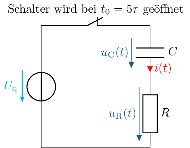
(a) Representation of the series connection consisting of a capacitance \(C\), a resistor \(R\) and a switch.

(b) Voltage and current curve over capacity at a DC voltage that is switched on at time \(t = 0\) and
switched off at time \(t_\mathrm {0}\).
Figure 7: The voltage and current curve over capacity. The diagram shows the reaction of the
capacitance to the sudden change in voltage and illustrates the typical charging behaviour.
The diagram 6b shows that despite the applied DC voltage \(U_\mathrm {q}\), the voltage \(u_\mathrm {c}(t)\) does not change simultaneously, but exhibits inertia. This time-varying behaviour is expressed in the circuit diagram 6a by the time-dependent variables \(u(t)\) and \(i(t)\).
In this example, the switch is closed at the start and is opened at \(t_0 = 5\tau \). The capacitor is not charged at the start. The diagram shows that, despite the applied voltage \(U_q\), the voltage across the capacitance \(u_C(t)\) does not change abruptly.
This switch-on behaviour results from the charging of the capacitance. To do this, the charge carriers must accumulate on the capacitor plates. This continues until the voltage between the plates corresponds to the voltage applied by the voltage source. Since the charge carriers required for charging must migrate into the capacitor plates, a corresponding current \(i_\mathrm {C}(t)\) flows during this process.
In the case of an ideally conductive circuit without ohmic resistance, the charge carriers would accumulate infinitely quickly on the capacitor plates, which would correspond to an infinitely high current. In reality, the capacitor or the lead to the capacitor has ohmic resistance, which slows down the charge carriers on their way to the capacitor plates, thus reducing the electric current. This results in the maximum possible current \(I_\mathrm {max}\).
\begin {equation} I_\mathrm {max} = \frac {U_\mathrm {q}}{R} \end {equation}
As soon as the switch is opened, the voltage across the capacitance is maintained. This means that the energy supplied remains in the capacitance and no longer changes in the steady state. Accordingly, no current flows when the capacitance is charged, which is equivalent to no-load operation in a steady-state DC network.
With the help of the two formulas 10 and 11, the behaviour of current and voltage at a capacitor is fully described, which now enables various calculations. Another example is the switching behaviour of a capacitor when a square-wave voltage is applied. The difference is that, unlike in example 6a, a constant voltage source is not switched via a switch, but rather the voltage source itself determines the input voltage.
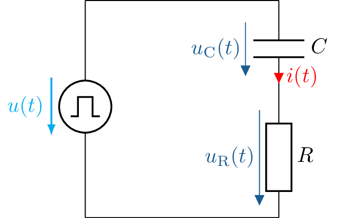
(a) Representation of the series connection consisting of a capacitance \(C\) and a resistance \(R\) at
a rectangular voltage source.
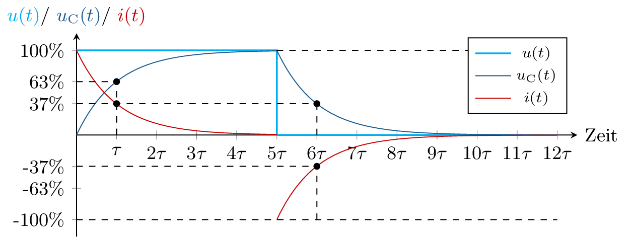
Figure 8: Voltage and current curve over capacity. The diagram shows the response of the
capacitance to a sudden change in voltage and illustrates the typical charging and discharging
behaviour of the capacitor.
In contrast to the switch, the voltage source in example 7a attempts to pull the system voltage to \(0\) from the point in time \(t_\mathrm {0} = 5\tau \). This leads to the capacitance being discharged. This results in an opposite current flow \(i_\mathrm {C}(t)\), as the charge carriers move away from the capacitor plates in order to return to a neutral state.
Capacity calculation
- Charge on plates \(Q = \sigma \cdot A = \varepsilon \cdot E \cdot A\)
- Calculate capacitance with \(C = \frac {\varepsilon \cdot A}{d}\)
- Stored energy \(W = \frac {1}{2} \cdot C \cdot V^2 \)
- Calculate the capacitance of two capacitors with different \(\varepsilon _{\mathrm {r}}\) over \(\vec {D}\)
