Knot- and Mesh analysis
When considering electrical networks, the currents in nodes and the voltages in meshes are analysed in particular. The analysis of nodes and meshes in electrical networks is carried out using the two Kirchhoff’s rules.
Learning objectives: Knot- and Mesh analysis
The Students
- 1.
- know the basic definitions for describing an electrical network.
- 2.
- can apply the node rule and the mesh rule to electrical networks.
1 Current density in free space
Facts and concepts from field theory lead to explanations in structured field space. To this end, Figure 1 shows a positively charged plate and a negatively charged plate facing each other.The space between the two plates has an electric field \(\vec {E}\) and a medium with conductivity \(\sigma \). Charge carriers can move in the free space. A directed movement of charge carriers and thus a current density \(\vec {J}\) between the plates occurs. The current density is source-free in the area under consideration.
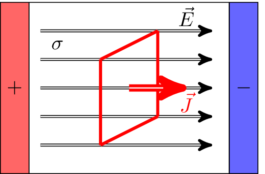
The source-free nature of the current density is illustrated by the equation 1. This describes that no sources or sinks exist, as there are no field-forming charges in space. In this case, the current density is source-free and the same number of charges flow into and out of the surface. Mathematically, this is expressed in the continuity equation for consideration in free space:
\begin {equation} \oint _{}^{} \vec {J} d\vec {A} = 0 \rightarrow div \vec {J} = 0 \label {divJQuellenfreiheit} \end {equation}
2 Current density in structured space
In a structured field space (see Figure 2), the current density must also be free of sources. All charges that enter the field space must also leave it again. This also applies in cases where an electrical conductor has more than one discharge path . A supply line with two conductors is indicated, in which the charges are distributed between the two conductors. The cylinder surface areas \(A_1\), \(A_2\) and \(A_3\) define a structured field space with the adjacent cylinders. Just as the charges are distributed, the current densities are distributed throughout the structured space. Thus, the current density \(\vec {J_1}\) is the sum of the outgoing current densities \(\vec {J_2}\) and \(\vec {J_3}\).
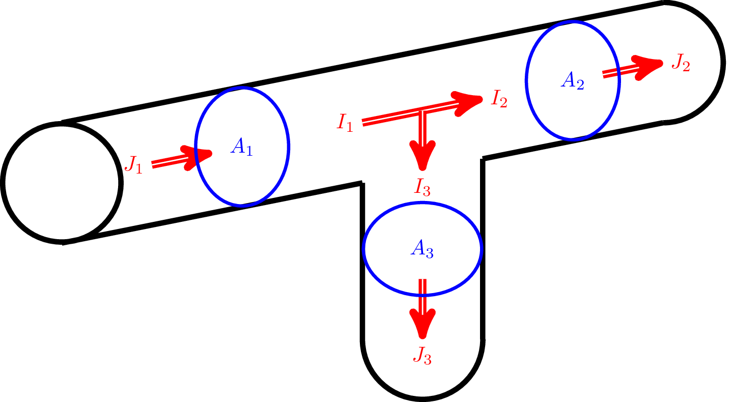
Since the field space in the example is structured by the surfaces and the cross-section of the conductor is defined, the currents of the conductors can be determined from the relationship between the current density and the surface area according to equation 2.
\begin {equation} I_1 = \iint _{A}^{} \vec {J_1} d\vec {A} \label {GleichungStromberechnung} \end {equation}
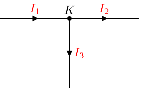
The relationship between the current densities can thus be transferred to the currents. The current of the supply line \(I_1\) is the sum of the two branch currents \(I_2\) and \(I_3\). The example conductor can also be represented as a simplified electrical network. The currents determined around the connection point K (node) are shown in Figure 3.
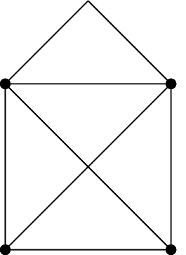
3 Digression: Graph theory
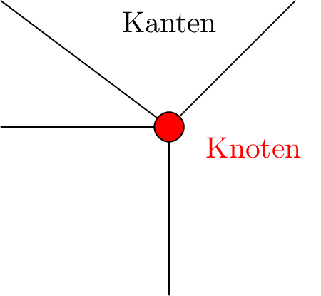
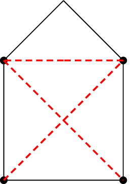
In mathematics, graph theory deals with the description of nodes and edges, while account analysis also defines nodes and branches. Graph theory allows the edges and nodes shown in Figure 4 and their properties to be related to each other. Multiple nodes can be connected to each other via the edges.
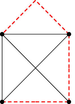
When several nodes are connected to each other with edges, a graph is created. This graph can be used to describe an electrical network, for example. The example of a network with five nodes and the edges between the nodes is shown in Figure 5. When searching for a path through the network , there are various possibilities. A path from node 1 via nodes 2, 4 and 5 back to node 1 is highlighted in red. If the start and end are the same node, this path is also referred to as a cycle in graph theory. Any cycle in which each node is "visitedönly once, except for the start and end, is called a "circle". In electrical networks, these circles are also referred to as meshes.
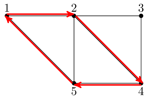
In mathematics, a matrix is a useful tool for explaining the relationship between nodes. The nodes have a differentiated number of edges, and not all nodes are connected to each other. The adjacency matrix describes the relationship between the nodes. Such an adjacency matrix is set up in equation 3 for the example network described. It thus completely describes the graph, apart from the graphical representation in the 2D display.
\begin {equation} A = \begin {bmatrix} \color {blue}{1} & 1 & 0 & 0 & 1\\ 1 & \color {blue}{1} & 1 & 1 & 1\\ 0 & 1 & \color {blue}{1} & 1 & 0\\ 0 & 1 & 1 & \color {blue}{1} & 1\\ 1 & 1 & 0 & 1 & \color {blue}{1} \end {bmatrix} \label {AdjazenzMatrix} \end {equation}
Key point: Graph theory
In graph theory, networks are described using edges and nodes. When analysing networks, paths and cycles are defined. A continuous cycle with an identical starting point and end point is referred to as a circle.
4 Knot, Branch, Mesh
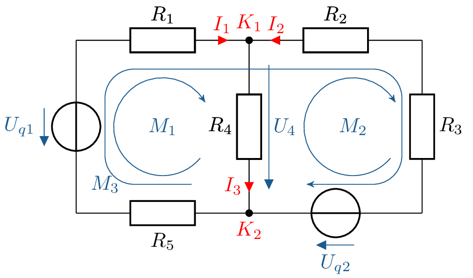
An electrical network consists of nodes, branches and meshes. A branch connects exactly two nodes by means of one or more circuit elements. The same current flows through all elements of a branch. There are three branches in Figure 6. One branch with the components \(R_1\), \(R_5\) and \(U_\mathrm {q1}\), one branch with the resistance \(R_4\) and one branch with the components \(R_2\), \(R_3\) and \(U_\mathrm {q2}\). A node is a point at which at least three connections of the circuit elements converge. The current can therefore split here. The electrical potential is identical for all connected terminals.
In the circuit diagram, a node is indicated by a filled circle. However, if two or more of these circles are connected to each other by only one line, it is a single node, since the potential is also the same here. A node is denoted by \(K_n\).
A mesh is a closed path consisting of at least two branches. In the net in Figure 6, three meshes can be defined:
- \(M_1\) consisting of \(R_1\), \(R_4\), \(R_5\) and \(U_\mathrm {q1}\)
- \(M_2\) consisting of \(R_2\), \(R_3\), \(R_4\) and \(U_\mathrm {q2}\)
- \(M_3\) consisting of \(R_1\), \(R_2\), \(R_3\), \(U_\mathrm {q2}\), \(R_5\) und \(U_\mathrm {q1}\)
A mesh is designated by \(M_\mathrm {n}\). The direction of rotation is important and is indicated by an arrow.
Key point: Knots, Branches and Meshes
Electrical networks are described by nodes, branches and meshes, analogous to graph theory.
5 The complete tree
For further analysis of the network, it is necessary to determine the network equations. However, this linear system of equations is always overdetermined, which is why it is necessary to reduce the number of equations. It is important to identify and eliminate the linearly dependent equations.
The nodes, branches and meshes of a network can be represented in a graph that only shows the connections between them. To represent the graph, all branches are shown as lines that connect the nodes. The content of the branch is irrelevant for this purpose. Figure 7 shows an example network with the resulting graph.
In this graph, a complete tree can be drawn that contains all nodes but does not itself form a mesh. The tree branches connect all nodes to each other but do not form a closed line. The tree branches can form branches, meaning that a node can also touch more than two tree branches. In larger networks, there are several possibilities for a complete tree, which are in principle equivalent. However, when presenting the various calculation methods, certain combinations are preferred depending on the method. A complete tree contains exactly \(k-1\) branches.
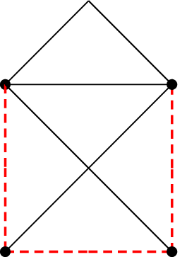
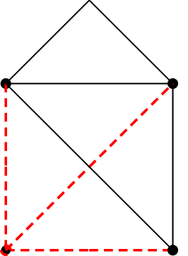
The branches belonging to the tree are called tree branches (red), the other connecting branches (black). To find the linearly independent meshes, a mesh is formed for each connecting branch that contains only tree branches except for the connecting branch.
- A network with \(z\) branches and \(k\) nodes contains \(z-k+1\) connecting branches.
Key point: The complete tree
With the help of a complete tree, all nodes are connected to each other by tree branches. This always results in k - 1 tree branches. The complete tree does not form a mesh.
6 Knot rule
If more than two lines meet at a point in an electrical network, this is referred to as a node K. The direction of the arrow from the perspective of the node determines the sign of the current. If a current flows into a node, the current arrow points towards the node and this is referred to as an inflow. If the current arrow points out of the node, the current flows out of the node and this is an outflow. The node analysis is based on Kirchhoff’s first law, which states: The sum of all currents at a node is zero. (Gleichung 4). This law follows directly from the continuity equation. (vgl. Abschnitt Current density in free space)
\begin {equation} \sum _{k = 1}^{N}{I_\mathrm {k} = 0} \label {Knotenregel} \end {equation}
Thus, for each node, the sum of the currents from inflows and outflows must balance each other out. Figure 9 shows a node K and the inflows and outflows. The flows \(I_1\) and \(I_2\) are inflows. The three flows \(I_3\), \(I_4\) and \(I_5\) are outflows.
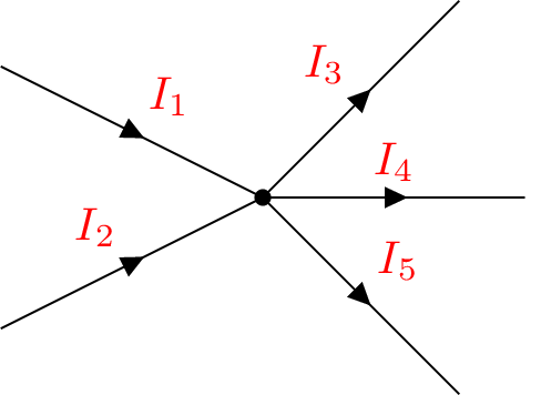
If the currents are applied one after the other and set to zero, the equation 5 is obtained. Depending on whether it is an inflow or an outflow, the sign is selected. Inflows are assigned a positive sign and outflows a negative sign.
\begin {equation} \sum _{k = 1}^{N}{I_\mathrm {k}} =0=I_1+I_2-I_3-I_4-I_5 \label {KnotenregelBeispielknoten} \end {equation}
Key point: Knot rule
7 Mesh rule
When a particle moves between two points in an electric field, work is done. If the starting point is identical to the end point, the same amount of work must be delivered as absorbed. In this case, the sum of the work is zero. If such a complete mesh cycle is performed along a closed path, the sum of the partial voltages must also be zero. This assumes that there is no time-varying magnetic flux density and therefore no electrical eddy field is created (see equation 7). The equation describes Faraday’s law of induction for static fields (here: no change in a magnetic field).
\begin {equation} \oint _{s}^{} \vec {E} d\vec {s} = 0 \rightarrow rot \vec {E} = 0 \label {GleichungRingintegralFeldstärke} \end {equation}
According to Kirchhoff’s second law, mesh analysis states that for a complete circuit (mesh) in an electrical network, the sum of all voltages is equal to zero. This is illustrated by the equation 8.
\begin {equation} \sum _{k = 1}^{N}{U_\mathrm {k}} =0 \label {Maschenregel} \end {equation}
Within a mesh, voltages with an arrow direction in the same direction are counted as positive, while voltages with an arrow direction opposite to the direction of rotation are counted as negative. Based on the current curves and potentials from Figure 10, the voltages of the respective branches can be determined. There is no potential difference above the parallel connection of the resistors. The same applies to the electrical connection below the parallel connection. The current \(I_\mathrm {R1}\) flows through the resistor \(R_\mathrm {1}\). According to Ohm’s law, this results in the voltage \(U_\mathrm {R1}\) across \(R_\mathrm {1}\). Equivalently, the voltage \(U_\mathrm {R2}\) across \(R_\mathrm {2}\) is determined.
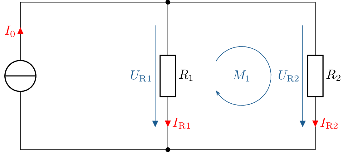
According to the network presented and the direction of the drawn mesh \(M_\mathrm {1}\), the relationship according to equation 9 applies. The voltage \(U_\mathrm {R2}\) runs in the same direction as the drawn mesh and is assigned a positive sign . The voltage \(U_\mathrm {R1}\) runs in the opposite direction to the mesh \(M_\mathrm {1}\) and is therefore negative. In total, these two voltages must add up to zero.
\begin {equation} \sum _\mathrm {k = 1}^{N}{U_\mathrm {k}} {= + U_\mathrm {R2}} {- U_\mathrm {R1}} {=0} \label {Maschengleichung} \end {equation}
Key point: Mesh rule
8 Knot and Mesh analysis
In node and mesh analysis, the complete system of equations consisting of node and mesh equations is set up and then solved. The procedure is simple, but generates a number of equations for a network that corresponds to the number of branches. The procedure is as follows:
- 1.
- Simplifying the network.
- 2.
- Draw all current arrows and create the graph.
- 3.
- Set up \(k-1\) node equations. Any node equation can be omitted, since in a network with \(k\) nodes only \(k-1\) node equations are linearly independent of each other. In principle, it does not matter which node equation is omitted. It is best to omit the most complicated equation.
- 4.
- Set up the \(m=z-k+1\) linearly independent mesh equations. The equations are created using the complete tree.
- 5.
- Solving the system of equations with the dimension \(z\).
- 6.
- If necessary, undo step 1.
The following example network is considered:
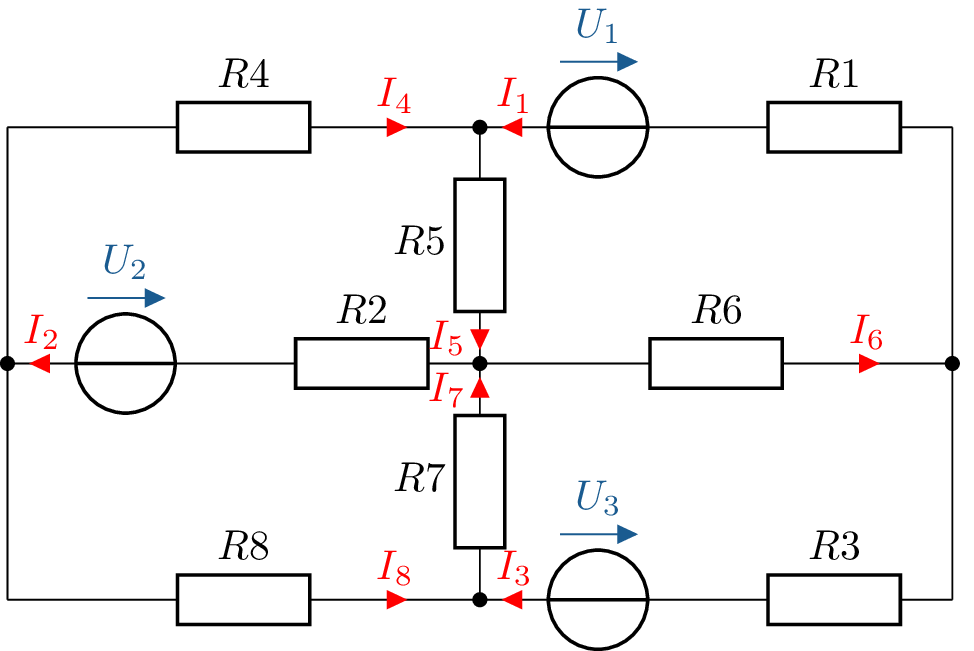
The corresponding graph and the meshes defined by it are shown in Figure 12. A different arrangement of the meshes is possible. As shown, meshes can also extend beyond branches.
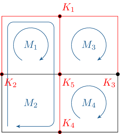
The network has \(z=8\) branches and \(k=5\) nodes. Therefore, \(k-1=4\) node equations and \(z-k+1=4\) mesh equations must be set up. Node 5 has four branches, the others only three. Therefore, the node equation for node 5 is omitted.
\begin {align*} K_1:\qquad & I_1+I_4-I_5=0\\ K_2:\qquad & I_2-I_4-I_8=0\\ K_3:\qquad & -I_1-I_3+I_6=0\\ K_4:\qquad & I_3-I_7+I_8=0\\ M_1:\qquad & R_2I_2 + R_4I_4 + R_5I_5 - U_{2} = 0\\ M_2:\qquad & R_4I_4 + R_5I_5 - R_7I_7 - R_8I_8 = 0\\ M_3:\qquad & -R_1I_1 - R_5I_5 - R_6I_6 + U_{1} = 0\\ M_4:\qquad & R_3I_3 + R_6I_6 + R_7I_7 - U_{3} = 0 \end {align*}
To make the system of equations easier to solve and to increase clarity, it can be represented in matrix notation. With a little practice, matrix notation can also be used immediately.
\begin {equation*} \left [\begin {array}{cccccccc} 1&0&0&1&-1&0&0&0\\ 0&1&0&-1&0&0&0&-1\\ -1&0&-1&0&0&1&0&0\\ 0&0&1&0&0&0&-1&1\\ 0&R_2&0&R_4&R_5&0&0&0\\ 0&0&0&R_4&R_5&0&-R_7&-R_8\\ -R_1&0&0&0&-R_5&-R_6&0&0\\ 0&0&R_3&0&0&R_6&R_7&0 \end {array}\right ] \cdot \left (\begin {array}{c} I_1\\I_2\\I_3\\I_4\\I_5\\I_6\\I_7\\I_8 \end {array}\right ) = \left (\begin {array}{c} 0\\0\\0\\0\\U_{2}\\0\\-U_{1}\\U_{3} \end {array}\right ) \end {equation*}
This 8th order system of equations can now in principle be solved using the methods known from mathematics. However, we do not want to do that here, as simpler methods are presented below that are easier to calculate.
Network analysis
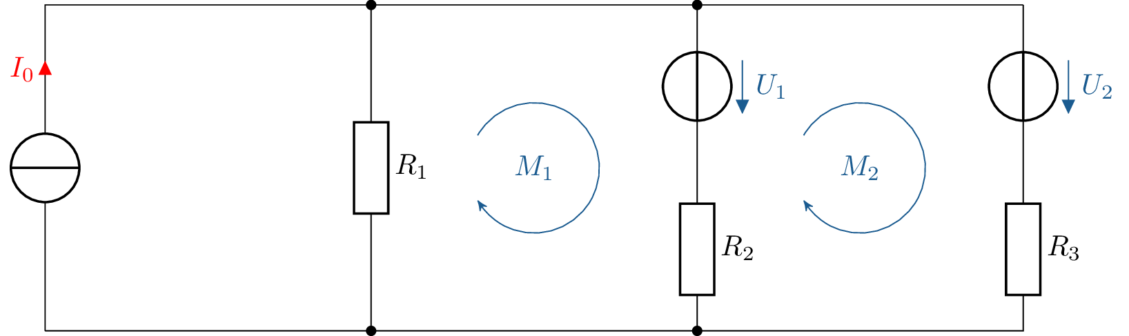
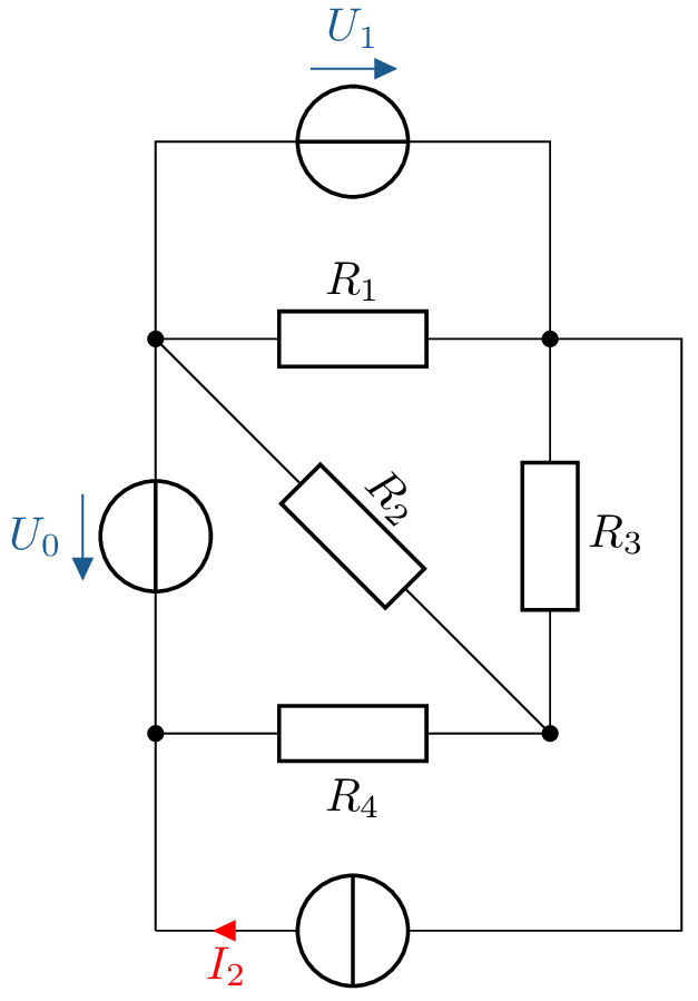
The electrical network shown in Figure 13 is given. The following tasks are to be completed:
-
- a)
- Plotting currents and voltages
- b)
- Setting up the node equations
- c)
- Setting up the mesh equation \(M_1\)
- d)
- Setting up the mesh equation \(M_2\) without the expression \(U_1\)
![PIC]()
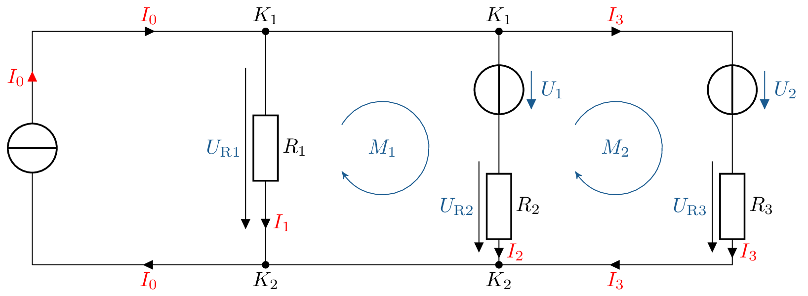
Figure 13: Example. Network analysis using Kirchhoff’s laws. - a)
- Specification of currents and voltages:
![PIC]()
- b)
- Knot equations: \begin {align} K_1: I_0-I_1-I_2-I_3&=0 \nonumber \\ K_2: -I_0+I_1+I_2+I_3&=0 \nonumber \end {align}
- c)
- Setting up the mesh equation \(M_1\) and \(M_2\): \begin {align} M_1: U_1+U_\mathrm {R2}-U_\mathrm {R1}&=0 \nonumber \\ M_2: U_2+U_\mathrm {R3}-U_\mathrm {R2}-U_1&=0 \nonumber \end {align}
- d)
- Setting up the mesh equation \(M_2\) without the expression \(U_1\) \begin {align} M_1: U_1&=U_\mathrm {R1}-U_\mathrm {R2} \nonumber \\ M_2: U_2+U_\mathrm {R3}-U_\mathrm {R2}-(U_\mathrm {R1}-U_\mathrm {R2})&=0 \nonumber \\ M_2: U_2+U_\mathrm {R3}-\cancel {U_\mathrm {R2}}-U_\mathrm {R1}+\cancel {U_\mathrm {R2}}&=0 \nonumber \\ M_2: U_2+U_\mathrm {R3}-U_\mathrm {R1}&=0 \nonumber \end {align}